Continuous Conditional Probability

[math] \newcommand{\NA}{{\rm NA}} \newcommand{\mat}[1]{{\bf#1}} \newcommand{\exref}[1]{\ref{##1}} \newcommand{\secstoprocess}{\all} \newcommand{\NA}{{\rm NA}} \newcommand{\mathds}{\mathbb}[/math]

In situations where the sample space is continuous we will follow the same procedure as in the previous section. Thus, for example, if [math]X[/math] is a continuous random variable with density function [math]f(x)[/math], and if [math]E[/math] is an event with positive probability, we define a conditional density function by the formula

[[math]] f(x|E) = \left \{ \matrix{ f(x)/P(E), & \mbox{if} \,\,x \in E, \cr 0, & \mbox{if}\,\,x \not \in E. \cr}\right. [[/math]]

Then for any event [math]F[/math], we have

[[math]] P(F|E) = \int_F f(x|E)\,dx\ . [[/math]]

The expression [math]P(F|E)[/math] is called the conditional probability of [math]F[/math] given [math]E[/math]. As in the previous section, it is easy to obtain an alternative expression for this probability:

[[math]] P(F|E) = \int_F f(x|E)\,dx = \int_{E\cap F} \frac {f(x)}{P(E)}\,dx = \frac {P(E\cap F)}{P(E)}\ . [[/math]]

We can think of the conditional density function as being 0 except on [math]E[/math], and normalized to have integral 1 over [math]E[/math]. Note that if the original density is a uniform density corresponding to an experiment in which all events of equal size are equally likely, then the same will be true for the conditional density.

Example In the spinner experiment (cf. Example), suppose we know that the spinner has stopped with head in the upper half of the circle, [math]0 \leq x \leq 1/2[/math]. What is the probability that [math]1/6 \leq x \leq 1/3[/math]? Here [math]E = [0,1/2][/math], [math]F = [1/6,1/3][/math], and [math]F \cap E = F[/math]. Hence

[[math]] \begin{eqnarray*} P(F|E) &=& \frac {P(F \cap E)}{P(E)} \\ &=& \frac {1/6}{1/2} \\ &=& \frac 13\ , \end{eqnarray*} [[/math]]

which is reasonable, since [math]F[/math] is 1/3 the size of [math]E[/math]. The conditional density function here is given by

[[math]] f(x|E) = \left \{ \matrix{ 2, & \mbox{if}\,\,\, 0 \leq x \lt 1/2, \cr 0, & \mbox{if}\,\,\, 1/2 \leq x \lt 1.\cr}\right. [[/math]]

Thus the conditional density function is nonzero only on [math][0,1/2][/math], and is uniform there.

Example In the dart game (cf. Example), suppose we know that the dart lands in the upper half of the target. What is the probability that its distance from the center is less than 1/2? Here [math]E = \{\,(x,y) : y \geq 0\,\}[/math], and [math]F = \{\,(x,y) : x^2 + y^2 \lt (1/2)^2\,\}[/math]. Hence,

[[math]] \begin{eqnarray*} P(F|E) & = & \frac {P(F \cap E)}{P(E)} = \frac {(1/\pi)[(1/2)(\pi/4)]} {(1/\pi)(\pi/2)} \\ & = & 1/4\ . \end{eqnarray*} [[/math]]

Here again, the size of [math]F \cap E[/math] is 1/4 the size of [math]E[/math]. The conditional density function is

[[math]] f((x,y)|E) = \left \{ \matrix{ f(x,y)/P(E) = 2/\pi, &\mbox{if}\,\,\,(x,y) \in E, \cr 0, &\mbox{if}\,\,\,(x,y) \not \in E.\cr}\right. [[/math]]

Example We return to the exponential density (cf. Example). We suppose that we are observing a lump of plutonium-239. Our experiment consists of waiting for an emission, then starting a clock, and recording the length of time [math]X[/math] that passes until the next emission. Experience has shown that [math]X[/math] has an exponential density with some parameter [math]\lambda[/math], which depends upon the size of the lump. Suppose that when we perform this experiment, we notice that the clock reads [math]r[/math] seconds, and is still running. What is the probability that there is no emission in a further [math]s[/math] seconds? Let [math]G(t)[/math] be the probability that the next particle is emitted after time [math]t[/math]. Then

[[math]] \begin{eqnarray*} G(t) & = & \int_t^\infty \lambda e^{-\lambda x}\,dx \\ & = & \left.-e^{-\lambda x}\right|_t^\infty = e^{-\lambda t}\ . \end{eqnarray*} [[/math]]

Let [math]E[/math] be the event “the next particle is emitted after time [math]r[/math]” and [math]F[/math] the event “the next particle is emitted after time [math]r + s[/math].” Then

[[math]] \begin{eqnarray*} P(F|E) & = & \frac {P(F \cap E)}{P(E)} \\ & = & \frac {G(r + s)}{G(r)} \\ & = & \frac {e^{-\lambda(r + s)}}{e^{-\lambda r}} \\ & = & e^{-\lambda s}\ . \end{eqnarray*} [[/math]]

This tells us the rather surprising fact that the probability that we have to wait [math]s[/math] seconds more for an emission, given that there has been no emission in [math]r[/math] seconds, is independent of the time [math]r[/math]. This property (called the memoryless property) was introduced in Example. When trying to model various phenomena, this property is helpful in deciding whether the exponential density is appropriate.

The fact that the exponential density is memoryless means that it is reasonable to assume if one comes upon a lump of a radioactive isotope at some random time, then the amount of time until the next emission has an exponential density with the same parameter as the time between emissions. A well-known example, known as the “bus paradox,” replaces the emissions by buses. The apparent paradox arises from the following two facts: 1) If you know that, on the average, the buses come by every 30 minutes, then if you come to the bus stop at a random time, you should only have to wait, on the average, for 15 minutes for a bus, and 2) Since the buses arrival times are being modelled by the exponential density, then no matter when you arrive, you will have to wait, on the average, for 30 minutes for a bus.

The reader can now see that in Exercises Exercise, Exercise, and Exercise, we were asking for simulations of conditional probabilities, under various assumptions on the distribution of the interarrival times. If one makes a reasonable assumption about this distribution, such as the one in Exercise, then the average waiting time is more nearly one-half the average interarrival time.

Independent Events

If [math]E[/math] and [math]F[/math] are two events with positive probability in a continuous sample space, then, as in the case of discrete sample spaces, we define [math]E[/math] and [math]F[/math] to be independent if [math]P(E|F) = P(E)[/math] and [math]P(F|E) = P(F)[/math]. As before, each of the above equations imply the other, so that to see whether two events are independent, only one of these equations must be checked. It is also the case that, if [math]E[/math] and [math]F[/math] are independent, then [math]P(E \cap F) = P(E)P(F)[/math].

Example In the dart game (see Example), let [math]E[/math] be the event that the dart lands in the upper half of the target ([math]y \geq 0[/math]) and [math]F[/math] the event that the dart lands in the right half of the target ([math]x \geq 0[/math]). Then [math]P(E \cap F)[/math] is the probability that the dart lies in the first quadrant of the target, and

[[math]] \begin{eqnarray*} P(E \cap F) & = & \frac 1\pi \int_{E \cap F} 1\,dxdy \\ & = & \mbox{Area}\,(E\cap F) \\ & = & \mbox{Area}\,(E)\,\mbox{Area}\,(F) \\ & = & \left(\frac 1\pi \int_E 1\,dxdy\right) \left(\frac 1\pi \int_F 1\,dxdy\right) \\ & = & P(E)P(F) \end{eqnarray*} [[/math]]

so that [math]E[/math] and [math]F[/math] are independent. What makes this work is that the events [math]E[/math] and [math]F[/math] are described by restricting different coordinates. This idea is made more precise\linebreak[4] below.

Joint Density and Cumulative Distribution Functions

In a manner analogous with discrete random variables, we can define joint density functions and cumulative distribution functions for multi-dimensional continuous random variables.

Definition

Let [math]X_1,~X_2, \ldots,~X_n[/math] be continuous random variables associated with an experiment, and let [math]{\bar X} = (X_1,~X_2, \ldots,~X_n)[/math]. Then the joint cumulative distribution function of [math]{\bar X}[/math] is defined by

[[math]] F(x_1, x_2, \ldots, x_n) = P(X_1 \le x_1, X_2 \le x_2, \ldots, X_n \le x_n)\ . [[/math]]

The joint density function of [math]{\bar X}[/math] satisfies the following equation:

[[math]] F(x_1, x_2, \ldots, x_n) = \int_{-\infty}^{x_1} \int_{-\infty}^{x_2} \cdots \int_{-\infty}^{x_n} f(t_1, t_2, \ldots t_n)\,dt_ndt_{n-1}\ldots dt_1\ . [[/math]]

It is straightforward to show that, in the above notation,

[[math]] \begin{equation} f(x_1, x_2, \ldots, x_n) = {{\partial^n F(x_1, x_2, \ldots, x_n)}\over {\partial x_1 \partial x_2 \cdots \partial x_n}}\ .\label{eq 4.4} \end{equation} [[/math]]

Independent Random Variables

As with discrete random variables, we can define mutual independence of continuous random variables.

Definition

Let [math]X_1, X_2, \ldots, X_n[/math] be continuous random variables with cumulative distribution functions [math]F_1(x),~F_2(x), \ldots,~F_n(x)[/math]. Then these random variables are mutually independent if

[[math]] F(x_1, x_2, \ldots, x_n) = F_1(x_1)F_2(x_2) \cdots F_n(x_n) [[/math]]

for any choice of [math]x_1, x_2, \ldots, x_n[/math]. Thus, if [math]X_1,~X_2, \ldots,~X_n[/math] are mutually independent, then the joint cumulative distribution function of the random variable [math]{\bar X} = (X_1, X_2, \ldots, X_n)[/math] is just the product of the individual cumulative distribution functions. When two random variables are mutually independent, we shall say more briefly that they are independent.

Using Equation \ref{eq 4.4}, the following theorem can easily be shown to hold for mutually independent continuous random variables.

Theorem

Let [math]X_1,X_2, \ldots,X_n[/math] be continuous random variables with density functions [math]f_1(x),~f_2(x), \ldots,~f_n(x)[/math]. Then these random variables are mutually independent if and only if

[[math]] f(x_1, x_2, \ldots, x_n) = f_1(x_1)f_2(x_2) \cdots f_n(x_n) [[/math]]

for any choice of [math]x_1,x_2, \ldots, x_n[/math].

Let's look at some examples.

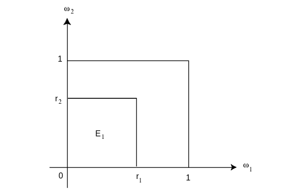
Example In this example, we define three random variables, [math]X_1,\ X_2[/math], and [math]X_3[/math]. We will show that [math]X_1[/math] and [math]X_2[/math] are independent, and that [math]X_1[/math] and [math]X_3[/math] are not independent. Choose a point [math]\omega = (\omega_1,\omega_2)[/math] at random from the unit square. Set [math]X_1 = \omega_1^2[/math], [math]X_2 = \omega_2^2[/math], and [math]X_3 = \omega_1 + \omega_2[/math]. Find the joint distributions [math]F_{12}(r_1,r_2)[/math] and [math]F_{23}(r_2,r_3)[/math]. We have already seen (see Example) that

[[math]] \begin{eqnarray*} F_1(r_1) & = & P(-\infty \lt X_1 \leq r_1) \\ & = & \sqrt{r_1}, \qquad \mbox{if} \,\,0 \leq r_1 \leq 1\ , \end{eqnarray*} [[/math]]

and similarly,

[[math]] F_2(r_2) = \sqrt{r_2}\ , [[/math]]

if [math]0 \leq r_2 \leq 1[/math]. Now we have (see Figure)

[math]X_1[/math] and [math]X_2[/math] are independent.

[[math]] \begin{eqnarray*} F_{12}(r_1,r_2) & = & P(X_1 \leq r_1 \,\, \mbox{and}\,\, X_2 \leq r_2) \\ & = & P(\omega_1 \leq \sqrt{r_1} \,\,\mbox{and}\,\, \omega_2 \leq \sqrt{r_2}) \\ & = & \mbox{Area}\,(E_1)\\ & = & \sqrt{r_1} \sqrt{r_2} \\ & = &F_1(r_1)F_2(r_2)\ . \end{eqnarray*} [[/math]]

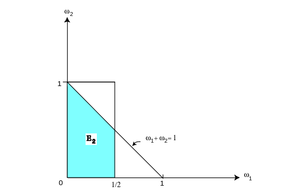
In this case [math]F_{12}(r_1,r_2) = F_1(r_1)F_2(r_2)[/math] so that [math]X_1[/math] and [math]X_2[/math] are independent. On the other hand, if [math]r_1 = 1/4[/math] and [math]r_3 = 1[/math], then (see [[#fig 5.16|Figure]])

[math]X_1[/math] and [math]X_3[/math] are not independent.

[[math]] \begin{eqnarray*} F_{13}(1/4,1) & = & P(X_1 \leq 1/4,\ X_3 \leq 1) \\ & = & P(\omega_1 \leq 1/2,\ \omega_1 + \omega_2 \leq 1) \\ & = & \mbox{Area}\,(E_2) \\ & = & \frac 12 - \frac 18 = \frac 38\ . \end{eqnarray*} [[/math]]

Now recalling that

[[math]] F_3(r_3) = \left \{ \matrix{ 0, & \mbox{if} \,\,r_3 \lt 0, \cr (1/2)r_3^2, & \mbox{if} \,\,0 \leq r_3 \leq 1, \cr 1-(1/2)(2-r_3)^2, & \mbox{if} \,\,1 \leq r_3 \leq 2, \cr 1, & \mbox{if} \,\,2 \lt r_3,\cr}\right. [[/math]]

(see Example), we have [math]F_1(1/4)F_3(1) = (1/2)(1/2) = 1/4[/math]. Hence, [math]X_1[/math] and [math]X_3[/math] are not independent random variables. A similar calculation shows that [math]X_2[/math] and [math]X_3[/math] are not independent either.

Although we shall not prove it here, the following theorem is a useful one. The statement also holds for mutually independent discrete random variables. A proof may be found in Rényi.

Theorem

Let [math]X_1, X_2, \ldots, X_n[/math] be mutually independent continuous random variables and let [math]\phi_1(x), \phi_2(x), \ldots, \phi_n(x)[/math] be continuous functions. Then [math]\phi_1(X_1),\phi_2(X_2), \ldots, \phi_n(X_n)[/math] are mutually independent.

Independent Trials

Using the notion of independence, we can now formulate for continuous sample spaces the notion of independent trials (see Definition).

Definition

A sequence [math]X_1, X_2, \dots, X_n[/math] of random variables [math]X_i[/math] that are mutually independent and have the same density is called an independent trials process.

As in the case of discrete random variables, these independent trials processes arise naturally in situations where an experiment described by a single random variable is repeated [math]n[/math] times.

Beta Density

We consider next an example which involves a sample space with both discrete and continuous coordinates. For this example we shall need a new density function called the beta density. This density has two parameters [math]\alpha[/math], [math]\beta[/math] and is defined by

[[math]] B(\alpha,\beta,x) = \left \{ \matrix{ (1/B(\alpha,\beta))x^{\alpha - 1}(1 - x)^{\beta - 1}, & {\mbox{if}}\,\, 0 \leq x \leq 1, \cr 0, & {\mbox{otherwise}}.\cr}\right. [[/math]]

Here [math]\alpha[/math] and [math]\beta[/math] are any positive numbers, and the beta function [math]B(\alpha,\beta)[/math] is given by the area under the graph of [math]x^{\alpha - 1}(1 - x)^{\beta - 1}[/math] between 0 and 1:

[[math]] B(\alpha,\beta) = \int_0^1 x^{\alpha - 1}(1 - x)^{\beta - 1}\,dx\ . [[/math]]

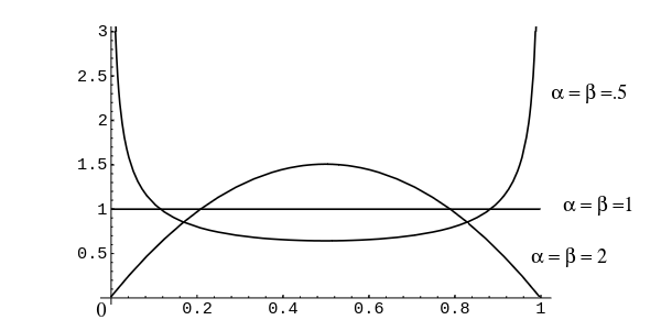
Note that when [math]\alpha = \beta = 1[/math] the beta density if the uniform density. When [math]\alpha[/math] and [math]\beta[/math] are greater than 1 the density is bell-shaped, but when they are less than 1 it is U-shaped as suggested by the examples in Figure.

Beta density for [math]\alpha = \beta = .5,1,2.[/math]

We shall need the values of the beta function only for integer values of [math]\alpha[/math] and [math]\beta[/math], and in this case

[[math]] B(\alpha,\beta) = \frac{(\alpha - 1)!\,(\beta - 1)!}{(\alpha + \beta - 1)!}\ . [[/math]]

Example In medical problems it is often assumed that a drug is effective with a probability [math]x[/math] each time it is used and the various trials are independent, so that one is, in effect, tossing a biased coin with probability [math]x[/math] for heads. Before further experimentation, you do not know the value [math]x[/math] but past experience might give some information about its possible values. It is natural to represent this information by sketching a density function to determine a distribution for [math]x[/math]. Thus, we are considering [math]x[/math] to be a continuous random variable, which takes on values between 0 and 1. If you have no knowledge at all, you would sketch the uniform density. If past experience suggests that [math]x[/math] is very likely to be near 2/3 you would sketch a density with maximum at 2/3 and a spread reflecting your uncertainly in the estimate of 2/3. You would then want to find a density function that reasonably fits your sketch. The beta densities provide a class of densities that can be fit to most sketches you might make. For example, for [math]\alpha \gt 1[/math] and [math]\beta \gt 1[/math] it is bell-shaped with the parameters [math]\alpha[/math] and [math]\beta[/math] determining its peak and its spread.

Assume that the experimenter has chosen a beta density to describe the state of his knowledge about [math]x[/math] before the experiment. Then he gives the drug to [math]n[/math] subjects and records the number [math]i[/math] of successes. The number [math]i[/math] is a discrete random variable, so we may conveniently describe the set of possible outcomes of this experiment by referring to the ordered pair [math](x, i)[/math].

We let [math]m(i|x)[/math] denote the probability that we observe [math]i[/math] successes given the value of [math]x[/math]. By our assumptions, [math]m(i|x)[/math] is the binomial distribution with probability [math]x[/math] for success:

[[math]] m(i|x) = b(n,x,i) = {n \choose i} x^i(1 - x)^j\ , [[/math]]

where [math]j = n - i[/math].

If [math]x[/math] is chosen at random from [math][0,1][/math] with a beta density [math]B(\alpha,\beta,x)[/math], then the density function for the outcome of the pair [math](x,i)[/math] is

[[math]] \begin{eqnarray*} f(x,i) & = & m(i|x)B(\alpha,\beta,x) \\ & = & {n \choose i} x^i(1 - x)^j \frac 1{B(\alpha,\beta)} x^{\alpha - 1}(1 - x)^{\beta - 1} \\ & = & {n \choose i} \frac 1{B(\alpha,\beta)} x^{\alpha + i - 1}(1 - x)^{\beta + j - 1}\ . \end{eqnarray*} [[/math]]

Now let [math]m(i)[/math] be the probability that we observe [math]i[/math] successes not knowing the value of [math]x[/math]. Then

[[math]] \begin{eqnarray*} m(i) & = & \int_0^1 m(i|x) B(\alpha,\beta,x)\,dx \\ & = & {n \choose i} \frac 1{B(\alpha,\beta)} \int_0^1 x^{\alpha + i - 1}(1 - x)^{\beta + j - 1}\,dx \\ & = & {n \choose i} \frac {B(\alpha + i,\beta + j)}{B(\alpha,\beta)}\ . \end{eqnarray*} [[/math]]

Hence, the probability density [math]f(x|i)[/math] for [math]x[/math], given that [math]i[/math] successes were observed, is

[[math]] f(x|i) = \frac {f(x,i)}{m(i)} [[/math]]

[[math]] \begin{equation} \ \ \ \ \ \ \ \ \ \ \ \ \ \ \ \ \ \ \ \ \ \ \ \ \ \ \ \ \ = \frac {x^{\alpha + i - 1}(1 - x)^{\beta + j - 1}}{B(\alpha + i,\beta + j)}\ ,\label{eq 4.5} \end{equation} [[/math]]

that is, [math]f(x|i)[/math] is another beta density. This says that if we observe [math]i[/math] successes and [math]j[/math] failures in [math]n[/math] subjects, then the new density for the probability that the drug is effective is again a beta density but with parameters [math]\alpha + i[/math], [math]\beta + j[/math].

Now we assume that before the experiment we choose a beta density with parameters [math]\alpha[/math] and [math]\beta[/math], and that in the experiment we obtain [math]i[/math] successes in [math]n[/math] trials. We have just seen that in this case, the new density for [math]x[/math] is a beta density with parameters [math]\alpha + i[/math] and [math]\beta + j[/math].

Now we wish to calculate the probability that the drug is effective on the next subject. For any particular real number [math]t[/math] between 0 and 1, the probability that [math]x[/math] has the value [math]t[/math] is given by the expression in Equation \ref{eq 4.5}. Given that [math]x[/math] has the value [math]t[/math], the probability that the drug is effective on the next subject is just [math]t[/math]. Thus, to obtain the probability that the drug is effective on the next subject, we integrate the product of the expression in Equation \ref{eq 4.5} and [math]t[/math] over all possible values of [math]t[/math]. We obtain:

[[math]] \begin{eqnarray*} \frac 1{B(\alpha + i,\beta + j)} \int_0^1 t\cdot t^{\alpha + i - 1}(1 - t)^{\beta + j - 1}\,dt & = & \frac {B(\alpha + i + 1,\beta + j)}{B(\alpha + i,\beta + j)} \\ & = & \frac {(\alpha + i)!\,(\beta + j - 1)!}{(\alpha + \beta + i + j)!} \cdot \frac {(\alpha + \beta + i + j - 1)!}{(\alpha + i - 1)!\,(\beta + j - 1)!} \\ & = & \frac {\alpha + i}{\alpha + \beta + n}\ . \end{eqnarray*} [[/math]]

If [math]n[/math] is large, then our estimate for the probability of success after the experiment is approximately the proportion of successes observed in the experiment, which is certainly a reasonable conclusion.

The next example is another in which the true probabilities are unknown and must be estimated based upon experimental data.

Example You are in a casino and confronted by two slot machines. Each machine pays off either 1 dollar or nothing. The probability that the first machine pays off a dollar is [math]x[/math] and that the second machine pays off a dollar is [math]y[/math]. We assume that [math]x[/math] and [math]y[/math] are random numbers chosen independently from the interval [math][0,1][/math] and unknown to you. You are permitted to make a series of ten plays, each time choosing one machine or the other. How should you choose to maximize the number of times that you win? One strategy that sounds reasonable is to calculate, at every stage, the probability that each machine will pay off and choose the machine with the higher probability. Let win([math]i[/math]), for [math]i = 1[/math] or 2, be the number of times that you have won on the [math]i[/math]th machine. Similarly, let lose([math]i[/math]) be the number of times you have lost on the [math]i[/math]th machine. Then, from Example, the probability [math]p(i)[/math] that you win if you choose the [math]i[/math]th machine is

[[math]] p(i) = \frac {{\mbox{win}}(i) + 1} {{\mbox{win}}(i) + {\mbox{lose}}(i) + 2}\ . [[/math]]

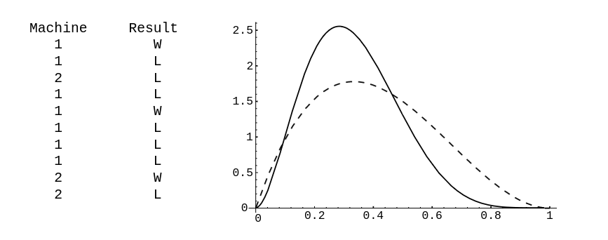
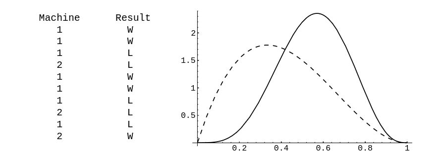
Thus, if [math]p(1) \gt p(2)[/math] you would play machine 1 and otherwise you would play machine 2. We have written a program TwoArm to simulate this experiment. In the program, the user specifies the initial values for [math]x[/math] and [math]y[/math] (but these are unknown to the experimenter). The program calculates at each stage the two conditional densities for [math]x[/math] and [math]y[/math], given the outcomes of the previous trials, and then computes [math]p(i)[/math], for [math]i = 1[/math], 2. It then chooses the machine with the highest value for the probability of winning for the next play. The program prints the machine chosen on each play and the outcome of this play. It also plots the new densities for [math]x[/math] (solid line) and [math]y[/math] (dotted line), showing only the current densities. We have run the program for ten plays for the case [math]x = .6[/math] and [math]y = .7[/math]. The result is shown in Figure.

Play the best machine.

The run of the program shows the weakness of this strategy. Our initial probability for winning on the better of the two machines is .7. We start with the poorer machine and our outcomes are such that we always have a probability greater than .6 of winning and so we just keep playing this machine even though the other machine is better. If we had lost on the first play we would have switched machines. Our final density for [math]y[/math] is the same as our initial density, namely, the uniform density. Our final density for [math]x[/math] is different and reflects a much more accurate knowledge about [math]x[/math]. The computer did pretty well with this strategy, winning seven out of the ten trials, but ten trials are not enough to judge whether this is a good strategy in the long run.

Play the winner.

Another popular strategy is the play-the-winner strategy. As the name suggests, for this strategy we choose the same machine when we win and switch machines when we lose. The program TwoArm will simulate this strategy as well. In Figure, we show the results of running this program with the play-the-winner strategy and the same true probabilities of .6 and .7 for the two machines. After ten plays our densities for the unknown probabilities of winning suggest to us that the second machine is indeed the better of the two. We again won seven out of the ten trials. Neither of the strategies that we simulated is the best one in terms of maximizing our average winnings. This best strategy is very complicated but is reasonably approximated by the play-the-winner strategy. Variations on this example have played an important role in the problem of clinical tests of drugs where experimenters face a similar situation.

General references

Doyle, Peter G. (2006). "Grinstead and Snell's Introduction to Probability". Retrieved June 6, 2024.