Central Limit Theorem for Continuous Independent Trials
We have seen in Central Limit Theorem for Continuous Independent Trials that the distribution function for the sum of a large number [math]n[/math] of independent discrete random variables with mean [math]\mu[/math] and variance [math]\sigma^2[/math] tends to look like a normal density with mean [math]n\mu[/math] and variance [math]n\sigma^2[/math]. What is remarkable about this result is that it holds for any distribution with finite mean and variance. We shall see in this section that the same result also holds true for continuous random variables having a common density function.
Let us begin by looking at some examples to see whether such a result is even plausible.
Standardized Sums
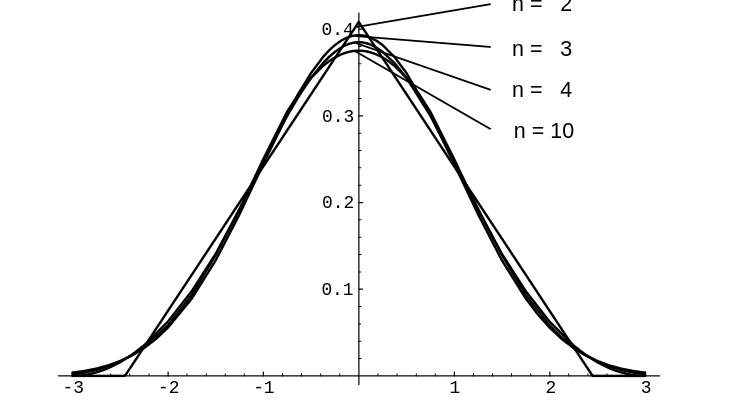
Example Suppose we choose [math]n[/math] random numbers from the interval [math][0,1][/math] with uniform density. Let [math]X_1[/math], [math]X_2[/math], \dots, [math]X_n[/math] denote these choices, and [math]S_n = X_1 + X_2 +\cdots+ X_n[/math] their sum. We saw in Example that the density function for [math]S_n[/math] tends to have a normal shape, but is centered at [math]n/2[/math] and is flattened out. In order to compare the shapes of these density functions for different values of [math]n[/math], we proceed as in the previous section: we standardize [math]S_n[/math] by defining
Then we see that for all [math]n[/math] we have
The density function for [math]S_n^*[/math] is just a standardized version of the density function for [math]S_n[/math] (see Figure).
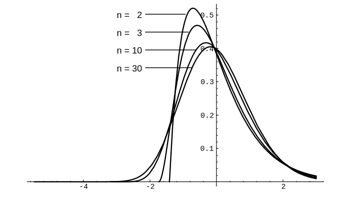
Example Let us do the same thing, but now choose numbers from the interval [math][0,+\infty)[/math] with an exponential density with parameter [math]\lambda[/math]. Then (see Example)
Here we know the density function for [math]S_n[/math] explicitly (see Sums of Continuous Random Variables). We can use Corollary to calculate the density function for [math]S_n^*[/math]. We obtain
The graph of the density function for [math]S_n^*[/math] is shown in Figure.

These examples make it seem plausible that the density function for the normalized random variable [math]S_n^*[/math] for large [math]n[/math] will look very much like the normal density with mean 0 and variance 1 in the continuous case as well as in the discrete case. The Central Limit Theorem makes this statement precise.
Central Limit Theorem
(Central Limit Theorem) Let [math]S_n = X_1 + X_2 +\cdots+ X_n[/math] be the sum of [math]n[/math] independent continuous random variables with common density function [math]p[/math] having expected value [math]\mu[/math] and variance [math]\sigma^2[/math]. Let [math]S_n^* = (S_n - n\mu)/\sqrt n \sigma[/math]. Then we have, for all [math]a \lt b[/math],
We shall give a proof of this theorem in Generating Functions for Continuous Densities. We will now look at some examples.
Example Suppose a surveyor wants to measure a known distance, say of 1 mile, using a transit and some method of triangulation. He knows that because of possible motion of the transit, atmospheric distortions, and human error, any one measurement is apt to be slightly in error. He plans to make several measurements and take an average. He assumes that his measurements are independent random variables with a common distribution of mean [math]\mu = 1[/math] and standard deviation [math]\sigma = .0002[/math] (so, if the errors are approximately normally distributed, then his measurements are within 1 foot of the correct distance about 65% of the time). What can he say about the average?
He can say that if [math]n[/math] is large, the average [math]S_n/n[/math] has a density function that is approximately normal, with mean [math]\mu = 1[/math] mile, and standard deviation [math]\sigma = .0002/\sqrt n[/math] miles. How many measurements should he make to be reasonably sure that his average lies within .0001 of the true value? The Chebyshev inequality says
so that we must have [math]n \ge 80[/math] before the probability that his error is less than .0001 exceeds .95.
We have already noticed that the estimate in the Chebyshev inequality is not
always a good one, and here is a case in point. If we assume that [math]n[/math] is large
enough so that the density for [math]S_n[/math] is approximately normal, then we have
and this last expression is greater than .95 if [math].5\sqrt{n} \ge 2.[/math] This says that it suffices to take [math]n = 16[/math] measurements for the same results. This second calculation is stronger, but depends on the assumption that [math]n = 16[/math] is large enough to establish the normal density as a good approximation to [math]S_n^*[/math], and hence to [math]S_n[/math]. The Central Limit Theorem here says nothing about how large [math]n[/math] has to be. In most cases involving sums of independent random variables, a good rule of thumb is that for [math]n \ge 30[/math], the approximation is a good one. In the present case, if we assume that the errors are approximately normally distributed, then the approximation is probably fairly good even for [math]n = 16[/math].
Estimating the Mean
Example Now suppose our surveyor is measuring an unknown distance with the same instruments under the same conditions. He takes 36 measurements and averages them. How sure can he be that his measurement lies within .0002 of the true value? Again using the normal approximation, we get
This means that the surveyor can be 99.7 percent sure that his average is within
.0002 of the true value. To improve his confidence, he can take more
measurements, or require less accuracy, or improve the quality of his
measurements (i.e., reduce the variance [math]\sigma^2[/math]). In each case, the Central
Limit Theorem gives quantitative information about the confidence of a
measurement process, assuming always that the normal approximation is valid.
Now suppose the surveyor does not know the mean or standard deviation of his
measurements, but assumes that they are independent. How should he proceed?
Again, he makes several measurements of a known distance and averages them. As before, the average error is approximately normally distributed, but now with unknown mean and variance.
Sample Mean
If he knows the variance [math]\sigma^2[/math] of the error distribution is .0002, then he can estimate the mean [math]\mu[/math] by taking the average, or sample mean of, say, 36 measurements:
where [math]n = 36[/math]. Then, as before, [math]E(\bar \mu) = \mu[/math]. Moreover, the preceding argument shows that
The interval [math](\bar \mu - .0002, \bar \mu + .0002)[/math] is called the 99.7% confidence interval for [math]\mu[/math] (see Example).
Sample Variance
If he does not know the variance [math]\sigma^2[/math] of the error distribution, then he can estimate [math]\sigma^2[/math] by the sample variance:
where [math]n = 36[/math]. The Law of Large Numbers, applied to the random variables [math](X_i - \bar \mu)^2[/math], says that for large [math]n[/math], the sample variance [math]\bar \sigma^2[/math] lies close to the variance [math]\sigma^2[/math], so that the surveyor can use [math]\bar \sigma^2[/math] in place of [math]\sigma^2[/math] in the argument above.
Experience has shown that, in most practical problems of this type, the sample
variance is a good estimate for the variance, and can be used in place of the
variance to determine confidence levels for the sample mean. This means that
we can rely on the Law of Large Numbers for estimating the variance, and the
Central Limit Theorem for estimating the mean.
We can check this in some special cases. Suppose we know that the error
distribution is normal, with unknown mean and variance. Then we can take
a sample of [math]n[/math] measurements, find the sample mean [math]\bar \mu[/math] and sample
variance [math]\bar \sigma^2[/math], and form
where [math]n = 36[/math]. We expect [math]T_n^*[/math] to be a good approximation for [math]S_n^*[/math] for large [math]n[/math].
[math]t[/math]-Density
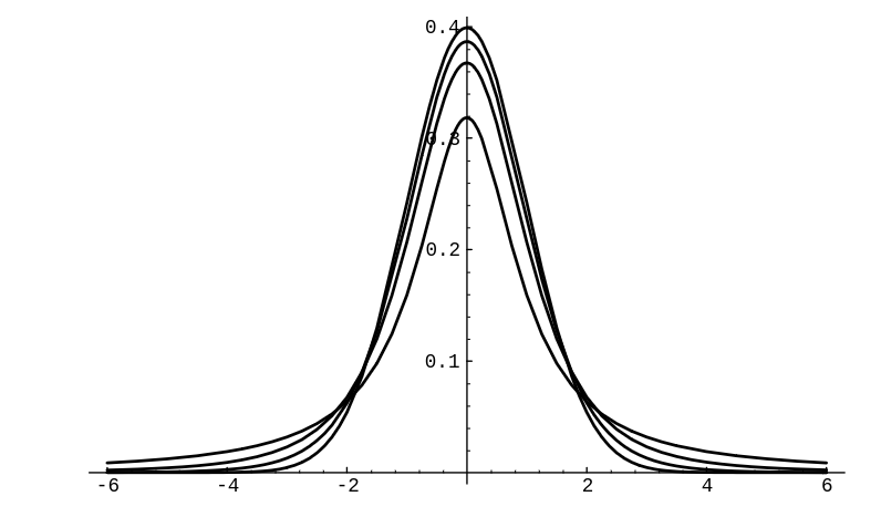
The statistician W. S. Gosset[Notes 1] has shown that in this case [math]T_n^*[/math] has a density function that is not normal but rather a [math]t[/math]-density with [math]n[/math] degrees of freedom. (The number [math]n[/math] of degrees of freedom is simply a parameter which tells us which [math]t[/math]-density to use.) In this case we can use the [math]t[/math]-density in place of the normal density to determine confidence levels for [math]\mu[/math]. As [math]n[/math] increases, the [math]t[/math]-density approaches the normal density. Indeed, even for [math]n = 8[/math] the [math]t[/math]-density and normal density are practically the same (see Figure).

Notes on computer problems:
-
[math]\ [/math]Simulation: Recall (see Corollary) that
[[math]] X = F^{-1}(rnd) [[/math]]will simulate a random variable with density [math]f(x)[/math] and distribution[[math]] F(X) = \int_{-\infty}^x f(t)\, dt\ . [[/math]]In the case that [math]f(x)[/math] is a normal density function with mean [math]\mu[/math] and standard deviation [math]\sigma[/math], where neither [math]F[/math] nor [math]F^{-1}[/math] can be expressed in closed form, use instead[[math]] X = \sigma\sqrt {-2\log(rnd)} \cos 2\pi(rnd) + \mu\ . [[/math]]
- [math]\ [/math]Bar graphs: you should aim for about 20 to 30 bars (of equal width) in your graph. You can achieve this by a good choice of the range [math][x{\rm min}, x{\rm min}][/math] and the number of bars (for instance, [math][\mu - 3\sigma, \mu + 3\sigma][/math] with 30 bars will work in many cases). Experiment!
General references
Doyle, Peter G. (2006). "Grinstead and Snell's Introduction to Probability" (PDF). Retrieved June 6, 2024.
