Comparison to ridge and Pandora's box

[math] \require{textmacros} \def \bbeta {\bf \beta} \def\fat#1{\mbox{\boldmath$#1$}} \def\reminder#1{\marginpar{\rule[0pt]{1mm}{11pt}}\textbf{#1}} \def\SSigma{\bf \Sigma} \def\ttheta{\bf \theta} \def\aalpha{\bf \alpha} \def\bbeta{\bf \beta} \def\ddelta{\bf \delta} \def\eeta{\bf \eta} \def\llambda{\bf \lambda} \def\ggamma{\bf \gamma} \def\nnu{\bf \nu} \def\vvarepsilon{\bf \varepsilon} \def\mmu{\bf \mu} \def\nnu{\bf \nu} \def\ttau{\bf \tau} \def\SSigma{\bf \Sigma} \def\TTheta{\bf \Theta} \def\XXi{\bf \Xi} \def\PPi{\bf \Pi} \def\GGamma{\bf \Gamma} \def\DDelta{\bf \Delta} \def\ssigma{\bf \sigma} \def\UUpsilon{\bf \Upsilon} \def\PPsi{\bf \Psi} \def\PPhi{\bf \Phi} \def\LLambda{\bf \Lambda} \def\OOmega{\bf \Omega} [/math]

Comparison to ridge

Here an inventory of the similarities and differences between the lasso and ridge regression estimators is presented. To recap what we have seen so far: both estimators optimize a loss function of the form and can be viewed as Bayesian estimators. But in various respects the lasso regression estimator exhibited differences from its ridge counterpart:

1. the former need not be uniquely defined (for a given value of the penalty parameter) whereas the latter is,
2. an analytic form of the lasso regression estimator does in general not exists,
3. but it is sparse (for large enough values of the lasso penalty parameter).

The remainder of this section expands this inventory.

Linearity

The ridge regression estimator is a linear (in the observations) estimator, while the lasso regression estimator is not. This is immediate from the analytic expression of the ridge regression estimator, [math]\hat{\bbeta}(\lambda_2) = (\mathbf{X}^{\top} \mathbf{X} + \lambda_2 \mathbf{I}_{pp})^{-1} \mathbf{X}^{\top} \mathbf{Y}[/math], which is a linear combination of the observations [math]\mathbf{Y}[/math]. To show the non-linearity of the lasso regression estimator available, it suffices to study the analytic expression of [math]j[/math]-th element of [math]\hat{\bbeta}(\lambda_1)[/math] in the orthonormal case: [math]\hat{\beta}_j(\lambda_1) = \mbox{sign}(\hat{\beta}_j) ( |\hat{\beta}_j| - \tfrac{1}{2} \lambda_1)_+ = \mbox{sign}(\mathbf{X}_{\ast,j}^{\top} \mathbf{Y} ) ( | \mathbf{X}_{\ast,j}^{\top} \mathbf{Y} | - \tfrac{1}{2} \lambda_1)_+[/math]. This clearly is not linear in [math]\mathbf{Y}[/math]. Consequently, the response [math]\mathbf{Y}[/math] may be scaled by some constant [math]c[/math], denoted [math]\tilde{\mathbf{Y}} = c \mathbf{Y}[/math], and the corresponding ridge regression estimators are one-to-one related by this same factor [math]\hat{\bbeta} (\lambda_2) = c \tilde{\bbeta} (\lambda_2)[/math]. The lasso regression estimator based on the unscaled data is not so easily recovered from its counterpart obtained from the scaled data.

Shrinkage

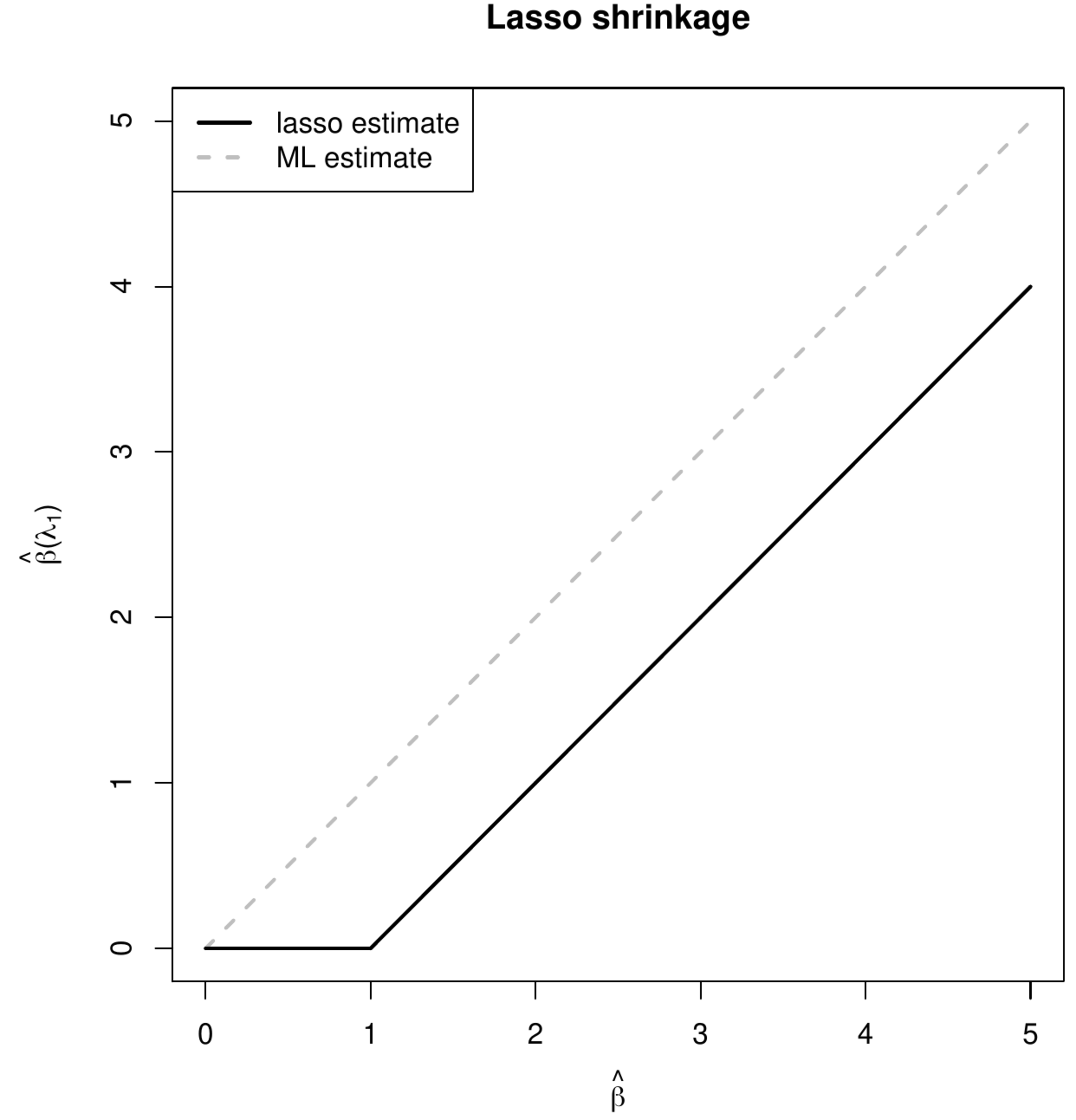
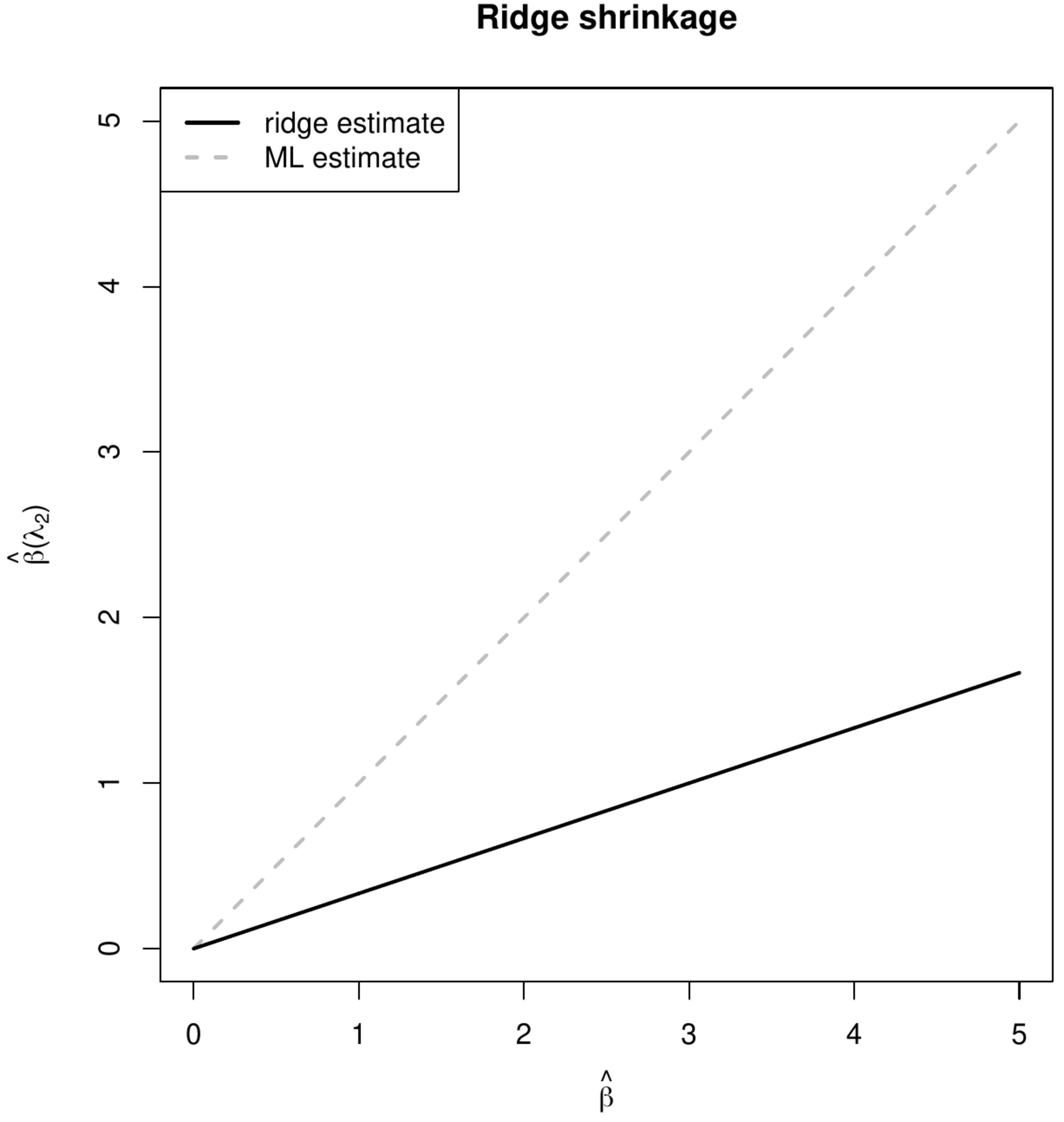
Both lasso and ridge regression estimation minimize the sum-of-squares plus a penalty. The latter encourages the estimator to be small, in particular closer to zero. This behavior is called shrinkage. The particular form of the penalty yields different types of this shrinkage behavior. This is best grasped in the case of an orthonormal design matrix. The [math]j[/math]-the element of the ridge regression estimator then is: [math]\hat{\beta}_j (\lambda_2) = (1+\lambda_2)^{-1} \hat{\beta}_j[/math], while that of the lasso regression estimator is: [math]\hat{\beta}_j (\lambda_1) = \mbox{sign}(\hat{\beta}_j) ( |\hat{\beta}_j| - \tfrac{1}{2} \lambda_1)_+[/math]. In Figure these two estimators [math]\hat{\beta}_j (\lambda_2)[/math] and [math]\hat{\beta}_j (\lambda_1)[/math] are plotted as a function of the maximum likelihood estimator [math]\hat{\beta}_j[/math]. Figure shows that lasso and ridge regression estimator translate and scale, respectively, the maximum likelihood estimator, which could also have been concluded from the analytic expression of both estimators. The scaling of the ridge regression estimator amounts to substantial and little shrinkage (in an absolute sense) for elements of the regression parameter [math]\bbeta[/math] with a large and small maximum likelihood estimate, respectively. In contrast, the lasso regression estimator applies an equal amount of shrinkage to each element of [math]\bbeta[/math], irrespective of the coefficients' sizes.

Solution path of the lasso estimator for data with an orthonormal design matrix.

Solution path of the ridge regression estimator for data with an orthonormal design matrix.

Simulation I: Covariate selection

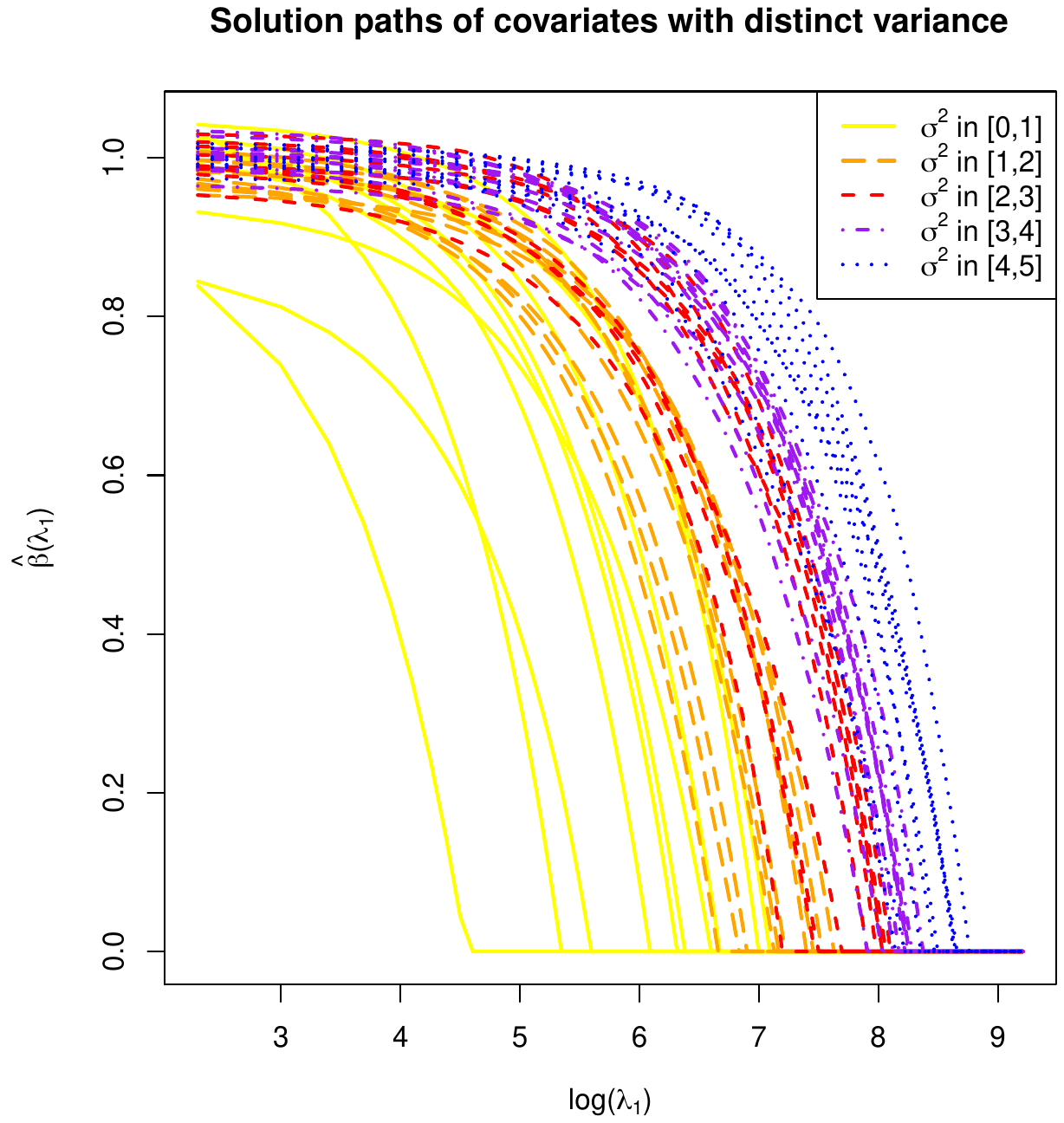
Here it is investigated whether lasso regression exhibits the same behaviour as ridge regression in the presence of covariates with differing variances. Recall: the simulation of Section Role of the variance of the covariates showed that ridge regression shrinks the estimates of covariates with a large spread less than those with a small spread. That simulation has been repeated, with the exact same parameter choices and sample size, but now with the ridge regression estimator replaced by the lasso regression estimator. To refresh the memory: in the simulation of Section Role of the variance of the covariates the linear regression model is fitted, now with the lasso regression estimator. The [math](n=1000) \times (p=50)[/math] dimensional design matrix [math]\mathbf{X}[/math] is sampled from a multivariate normal distribution: [math]\mathbf{X}_{i,\ast}^{\top} \sim \mathcal{N}(\mathbf{0}_{50}, \mathbf{\Sigma})[/math] with [math]\mathbf{\Sigma}[/math] diagonal and [math](\mathbf{\Sigma})_{jj} = j / 10[/math] for [math]j=1, \ldots, p[/math]. The response [math]\mathbf{Y}[/math] is generated through [math]\mathbf{Y} = \mathbf{X} \bbeta + \vvarepsilon[/math] with [math]\bbeta[/math] a vector of all ones and [math]\vvarepsilon[/math] sampled from the multivariate standard normal distribution. Hence, all covariates contribute equally to the response.

Regularization paths of the lasso regression estimator related to the simulations presented in Section Simulation I: Covariate selection

Regularization paths of the lasso regression estimator related to the simulations presented in Section Simulation II: correlated covariates

The results of the simulation are displayed in Figure, which shows the regularization paths of the [math]p=50[/math] covariates. The regularization paths are demarcated by color and style to indicate the size of the spread of the corresponding covariate. These regularization paths show that the lasso regression estimator shrinks -- like the ridge regression estimator -- the covariates with the smallest spread most. For the lasso regression this translates (for sufficiently large values of the penalty parameter) into a preference for the selection of covariates with largest variance.

Intuition for this behavior of the lasso regression estimator may be obtained through geometrical arguments analogous to that provided for the similar behaviour of the ridge regression estimator in Section Role of the variance of the covariates . Algebraically it is easily seen when assuming an orthonormal design with [math]\mbox{Var}(X_1) \gg \mbox{Var}(X_2)[/math]. The lasso regression loss function can then be rewritten, as in Example, to:

[[math]] \begin{eqnarray*} \| \mathbf{Y} - \mathbf{X} \bbeta \|_2^2 + \lambda_1 \| \bbeta \|_1 & = & \| \mathbf{Y} - \tilde{\mathbf{X}} \ggamma \|_2^2 + \lambda_1 [\mbox{Var}(X_1)]^{-1/2} | \gamma_1 | + \lambda_1 [\mbox{Var}(X_2)]^{-1/2} | \gamma_2 |, \end{eqnarray*} [[/math]]

where [math]\gamma_1 = [\mbox{Var}(X_1)]^{1/2} \beta_1[/math] and [math]\gamma_2 = [\mbox{Var}(X_2)]^{1/2} \beta_2[/math]. The rescaled design matrix [math]\tilde{\mathbf{X}}[/math] is now orthonormal and analytic expressions of estimators of [math]\gamma_1[/math] and [math]\gamma_2[/math] are available. The former parameter is penalized substantially less than the latter as [math]\lambda_1 [\mbox{Var}(X_1)]^{-1/2} \ll \lambda_1 [\mbox{Var}(X_2)]^{-1/2}[/math]. As a result, if for large enough values of [math]\lambda_1[/math] one variable is selected, it is more likely to be [math]\gamma_1[/math].

Simulation II: correlated covariates

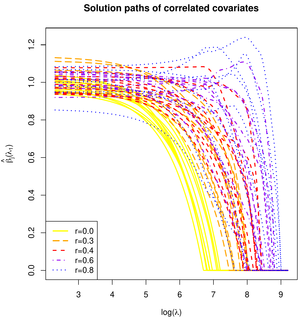
The behaviour of the lasso regression estimator is now studied in the presence of collinearity among the covariates. Previously, in simulation, Section Ridge regression and collinearity , the ridge regression estimator was shown to exhibit the joint shrinkage of strongly collinear covariates. This simulation is repeated for the lasso regression estimator. The details of the simulation are recapped. The linear regression model is fitted by means of the lasso regression estimator. The [math](n=1000) \times (p=50)[/math] dimensional design matrix [math]\mathbf{X}[/math] is samples from a multivariate normal distribution: [math]\mathbf{X}_{i,\ast}^{\top} \sim \mathcal{N}(\mathbf{0}_{50}, \mathbf{\Sigma})[/math] with a block-diagonal [math]\mathbf{\Sigma}[/math]. The [math]k[/math]-the, [math]k=1,\ldots,5[/math], diagonal block, denoted [math]\mathbf{\Sigma}_{kk}[/math] comprises ten covariates and equals [math]\frac{k-1}{5} \, \mathbf{1}_{10 \times 10} + \frac{6-k}{5} \, \mathbf{I}_{10 \times 10}[/math] for [math]k=1, \ldots, 5[/math]. The response vector [math]\mathbf{Y}[/math] is then generated by [math]\mathbf{Y} = \mathbf{X} \bbeta + \vvarepsilon[/math], with [math]\vvarepsilon[/math] sampled from the multivariate standard normal distribution and [math]\bbeta[/math] containing only ones. Again, all covariates contribute equally to the response.

The results of the above simulation results are captured in Figure. It shows the lasso regularization paths for all elements of the regression parameter [math]\bbeta[/math]. The regularization paths of covariates corresponding to the same block of [math]\mathbf{\Sigma}[/math] (indicative of the degree of collinearity) are now marcated by different colors and styles. Whereas the ridge regularization paths nicely grouped per block, the lasso counterparts do not. The selection property spoils the party. Instead of shrinking the regression parameter estimates of collinear covariates together, the lasso regression estimator (for sufficiently large values of its penalty parameter [math]\lambda_1[/math]) tends to pick one covariates to enters the model while forcing the others out (by setting their estimates to zero).

Pandora's box

Many variants of penalized regression, in particular of lasso regression, have been presented in the literature. Here we give an overview of some of the more current ones. Not a full account is given, but rather a brief introduction with emphasis on their motivation and use.

Elastic net

The elastic net regression estimator is a modication of the lasso regression estimator that preserves its strength and harnesses its weaknesses. The biggest appeal of the lasso regression estimator is clearly its ability to perform selection. Less pleasing are

1. the non-uniquess of the lasso regression estimator due to the non-strict convexity of its loss function,
2. the bound on the number of selected variables, i.e. maximally [math]\min \{ n, p \}[/math] can be selected,
3. and the observation that strongly (positively) collinear covariates are not shrunken together: the lasso regression estimator selects among them while it is hard to distinguish their contributions to the variation of the response. While it does not select, the ridge regression estimator does not exhibit these less pleasing features.

These considerations led to combine the strengths of the lasso and ridge regression estimators and form a ‘best-of-both-worlds’ estimator, called the elastic net regression estimator, defined as:

[[math]] \begin{eqnarray*} \hat{\bbeta}(\lambda_1, \lambda_2) & = & \arg \min_{\bbeta \in \mathbb{R}^p} \| \mathbf{Y} - \mathbf{X} \bbeta \|_2^2 + \lambda_1 \| \bbeta \|_1 + \tfrac{1}{2} \lambda_2 \| \bbeta \|_2^2. \end{eqnarray*} [[/math]]

The elastic net penalty -- defined implicitly in the preceeding display -- is thus simply a linear combination of the lasso and ridge penalties. Consequently, the elastic net regression estimator encompasses its lasso and ridge counterparts. Hereto just set [math]\lambda_2=0[/math] or [math]\lambda_1=0[/math], respectively. A novel estimator is defined when both penalties act simultaneously, i.e. when their corresponding penalty parameters are both nonzero.

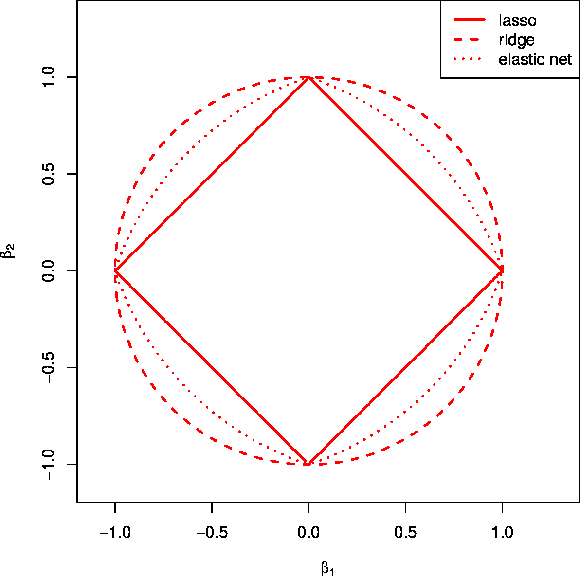
Does this novel elastic net estimator indeed inherit the strengths of the lasso and ridge regression estimators? Let us turn to the aforementioned motivation behind the elastic net estimator. Starting with the uniqueness, the strict convexity of the ridge penalty renders the elastic net loss function strictly convex, as it is a combination of the ridge penalty and the lasso function -- notably non-strict convex when the dimension [math]p[/math] exceeds the sample size [math]n[/math]. This warrants the existence of a unique minimizer of the elastic net loss function. To assess the preservation of the selection property, now without the bound on the maximum number of selectable variables, exploit the equivalent constraint estimation formulation of the elastic net estimator. Figure shows the parameter constraint of the elastic net estimator for the ‘[math]p=2[/math]’-case, which is defined by the set:

[[math]] \begin{eqnarray*} \{(\beta_1, \beta_2) \in \mathbb{R}^2 \, : \, \lambda_1 (| \beta_1 | + | \beta_2 |) + \tfrac{1}{2} \lambda_2 (\beta_1^2 + \beta_2^2) \leq c(\lambda_1, \lambda_2) \}. \end{eqnarray*} [[/math]]

Visually, the ‘elastic net parameter constraint’ is a comprise between the circle and the diamond shaped constraints of the ridge and lasso regression estimators. This compromise inherits exactly the right geometrical features: the strict convexity of the ‘ridge circle’ and the ‘corners’ (referring to points at which the constraint's boundary is non-smootness/non-differentiability) falling at the axes of the ‘lasso constraint’. The latter feature, by the same argumentation as presented in Section Sparsity , endows the elastic net estimator with the selection property. Moreover, it can -- in principle -- select [math]p[/math] features as the point in the parameter space where the smallest level set of the unpenalized loss hits the elastic net parameter constraint need not fall on any axis. For example, in the ‘[math]p=2, n=1[/math]’-case the level sets of the sum-of-squares loss are straight lines that, when almost parallel to the edges of the ‘lasso diamond’, are unlikely to first hit the elastic net parameter constraint at one of its corners. Finally, the largest penalty parameter relates (reciprocally) to the volume of the elastic net parameter constraint, while the ratio between [math]\lambda_1[/math] and [math]\lambda_2[/math] determines whether it is closer to the ‘ridge circle’ or to the ‘lasso diamond’.

The left panel depicts the parameter constraint induced by the elastic net penalty and, for reference, those of the lasso and ridge are added.

The right panel shows the contour plot of the cross-validated loglikelihood vs. the two penalty parameters of the elastic net estimator.

Whether the elastic net regression estimator also delivers on the joint shrinkage property is assessed by simulation (not shown). The impression given by these simulations is that the elastic net has joint shrinkage potential. This, however, usually requires a large ridge penalty, which then dominates the elastic net penalty.

The elastic net regression estimator can be found with procedures similar to those that evaluate the lasso regression estimator (see Section Estimation ) as the elastic net loss can be reformulated as a lasso loss. Hereto the ridge part of the elastic net penalty is absorbed into the sum of squares using the data augmentation trick of Exercise Exercise which showed that the ridge regression estimator is the ML regression estimator of the related regression model with [math]p[/math] zeros and rows added to the response and design matrix, respectively. That is, write [math]\tilde{\mathbf{Y}} = (\mathbf{Y}^{\top}, \mathbf{0}_{p}^{\top})^{\top}[/math] and [math]\tilde{\mathbf{X}} = (\mathbf{X}^{\top}, \sqrt{\lambda_2} \, \mathbf{I}_{pp})^{\top}[/math]. Then:

[[math]] \begin{eqnarray*} \| \tilde{\mathbf{Y}} - \tilde{\mathbf{X}} \bbeta \|_2^2 & = & \| \mathbf{Y} - \mathbf{X} \beta \|_2^2 + \lambda_2 \| \bbeta \|_2^2. \end{eqnarray*} [[/math]]

Hence, the elastic net loss function can be rewritten to [math]\| \tilde{\mathbf{Y}} - \tilde{\mathbf{X}} \bbeta \|_2^2 + \lambda_1 \| \bbeta \|_1[/math]. This is familiar territory and the lasso algorithms of Section Estimation can be used. present a different algorithm for the evaluation of the elastic net estimator that is faster and numerically more stable (see also [[exercise:2295037c70 |Exercise]). Irrespectively, the reformulation of the elastic net loss in terms of augmented data also reveals that the elastic net regression estimator can select [math]p[/math] variables. Even for [math]p \gt n[/math], which is immediate from the observation that [math]\mbox{rank}(\tilde{\mathbf{X}})=p[/math].

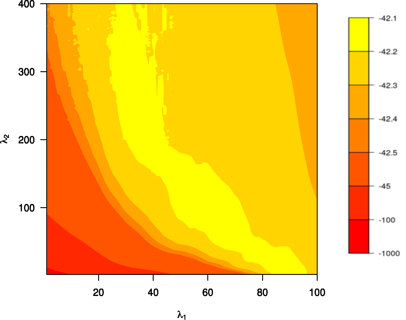
The penalty parameters need tuning, e.g. by cross-validation. They are subject to empirically indeterminancy. That is, often a large range of [math](\lambda_1, \lambda_2)[/math]-combinations will yield a similar cross-validated performance as can be witnessed from Figure. It shows the contourplot of the penalty parameters vs. this performance. There is a yellow ‘banana-shaped’ area that corresponds to the same and optimal performance. Hence, no single [math](\lambda_1, \lambda_2)[/math]-combination can be distinguished as all yield the best performance. This behaviour may be understood intuitively. Reasoning loosely, while the lasso penalty [math]\lambda_1 \| \bbeta \|_1[/math] ensures the selection property and the ridge penalty [math]\tfrac{1}{2} \lambda_2 \| \bbeta \|_2^2[/math] warrants the uniqueness and joint shrinkage of coefficients of collinear covariates, they have a similar effect on the size of the estimator. Both shrink, although in different norms. But a reduction in the size of [math]\hat{\bbeta}(\lambda_1, \lambda_2)[/math] in one norm implies a reduction in another. An increase in either the lasso and ridge penalty parameter will have a similar effect on the elastic net estimator: it shrinks. The selection and ‘joint shrinkage’ properties are only consequences of the employed penalty and are not criteria in the optimization of the elastic net loss function. There, only size matters. The size of [math]\bbeta[/math] refers to [math]\lambda_1 \| \bbeta \|_1 + \tfrac{1}{2} \lambda_2 \| \bbeta \|_2^2[/math]. As in the size the lasso and ridge penalties appear as a linear combination in the elastic net loss function and have a similar effect on the elastic net estimator: there are many positive [math](\lambda_1, \lambda_2)[/math]-combinations that constrain the size of the elastic net estimator equally. In contrast, for both the lasso and ridge regression estimators, different penalty parameters yield estimators of different sizes (defined accordingly). Moreover, it is mainly the size that determines the cross-validated performance as the size determines the shrinkage of the estimator and, consequently, the size of the errors. But only a fixed size leaves enough freedom to distribute this size over the [math]p[/math] elements of the regression parameter estimator [math]\hat{\bbeta}(\lambda_1, \lambda_2)[/math] and, due to the collinearity, among them many that yield a comparable performance. Hence, if a particularly sized elastic net estimator [math]\hat{\bbeta}(\lambda_1, \lambda_2)[/math] optimizes the cross-validated performance, then high-dimensionally there are likely many others with a different [math](\lambda_1, \lambda_2)[/math]-combination but of equal size and similar performance.

The empirical indeterminancy of penalty parameters touches upon another issues. In principle, the elastic net regression estimator can decide whether a sparse or non-sparse solution is most appropriate. The indeterminancy indicates that for any sparse elastic net regression estimator a less sparse one can be found with comparable performance, and vice versa. Care should be exercised when concluding on the sparsity of the linear relation under study from the chosen elastic net regression estimator.

A solution to the indeterminancy of the optimal penalty parameter combination is to fix their ratio. For interpretation purposes this is done through the introduction of a ‘mixing parameter’ [math]\alpha \in [0,1][/math]. The elastic net penalty is then written as [math]\lambda [ \alpha \| \bbeta \|_1 + \tfrac{1}{2} (1-\alpha) \| \bbeta \|_2^2 ][/math]. The mixing parameter is set by the user while [math]\lambda \gt 0[/math] is typically found through cross-validation (cf. the implementation in the glmnet-package) . Generally, no guidance on the choice of mixing parameter [math]\alpha[/math] can be given. In fact, it is a tuning parameter and as such needs tuning rather then setting out of the blue.

Fused lasso

The fused lasso regression estimator proposed by is the counterpart of the fused ridge regression estimator encountered in Example. It is a generalization of the lasso regression estimator for situations where the order of index [math]j[/math], [math]j=1, \ldots, p[/math], of the covariates has a certain meaning such as a spatial or temporal one. The fused lasso regression estimator minimizes the sum-of-squares augmented with the lasso penalty, the sum of the absolute values of the elements of the regression parameter, and the [math]\ell_1[/math]-fusion (or simply fusion if clear from the context) penalty, the sum of the first order differences of the regression parameter. Formally, the fused lasso estimator is defined as:

[[math]] \begin{eqnarray*} \hat{\bbeta} (\lambda_1, \lambda_{1,f}) & =& \arg \min_{\bbeta \in \mathbb{R}^p} \| \mathbf{Y} - \mathbf{X} \bbeta \|_2^2 + \lambda_1 \| \bbeta \|_{1} + \lambda_{1,f} \sum\nolimits_{j=2}^{p} | \beta_{j} - \beta_{j-1} |, \end{eqnarray*} [[/math]]

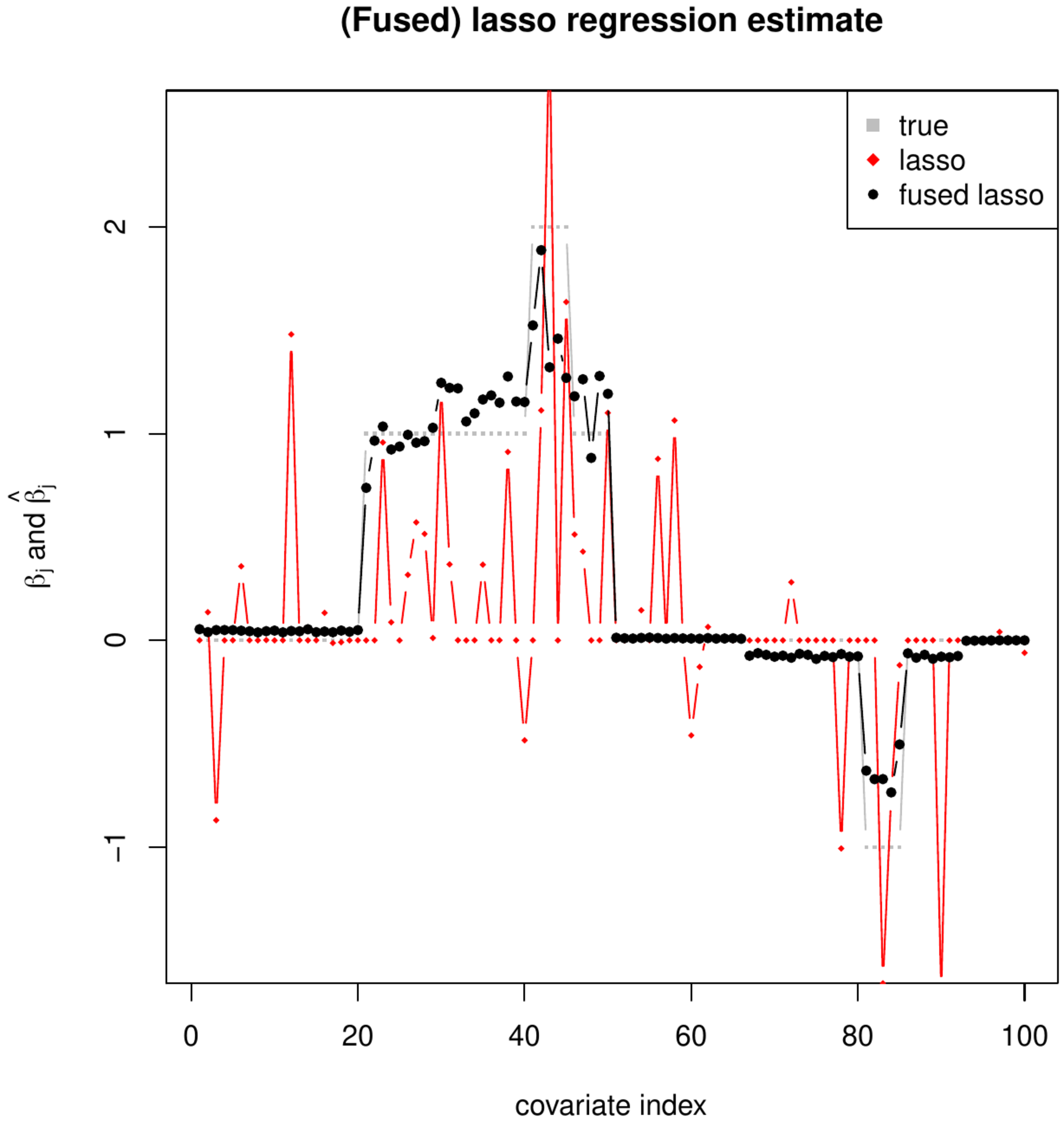
which involves two penalty parameters [math]\lambda_{1}[/math] and [math]\lambda_{1,f}[/math] for the lasso and fusion penalties, respectively. As a result of adding the fusion penalty the fused lasso regression estimator not only shrinks elements of [math]\bbeta[/math] towards zero but also the difference of neighboring elements of [math]\bbeta[/math]. In particular, for large enough values of the penalty parameters the estimator selects elements of and differences of neighboring elements of [math]\bbeta[/math]. This corresponds to a sparse estimate of [math]\bbeta[/math] while the vector of its first order differences too is dominated by zeros. That is many elements of [math]\hat{\bbeta} (\lambda_1, \lambda_{1,f})[/math] equal zero with few changes in [math]\hat{\bbeta} (\lambda_1, \lambda_{1,f})[/math] when running over [math]j[/math]. Hence, the fused lasso regression penalty encourages large sets of neighboring elements of [math]j[/math] to have a common (or at least a comparable) regression parameter estimate. This is visualized -- using simulated data from a simple toy model with details considered irrelevant for the illustration -- in Figure where the elements of the fused lasso regression estimate [math]\hat{\bbeta} (\lambda_1, \lambda_{1,f})[/math] are plotted against the index of the covariates. For reference the true [math]\bbeta[/math] and the lasso regression estimate with the same [math]\lambda_1[/math] are added to the plot. Ideally, for a large enough fusion penalty parameter, the elements of [math]\hat{\bbeta} (\lambda_1, \lambda_{1,f})[/math] would form a step-wise function in the index [math]j[/math], with many equalling zero and exhibiting few changes, as the elements of [math]\bbeta[/math] do. While this is not the case, it is close, especially in comparison to the elements of its lasso cousin [math]\hat{\bbeta}(\lambda_1)[/math], thus showing the effect of the inclusion of the fusion penalty.

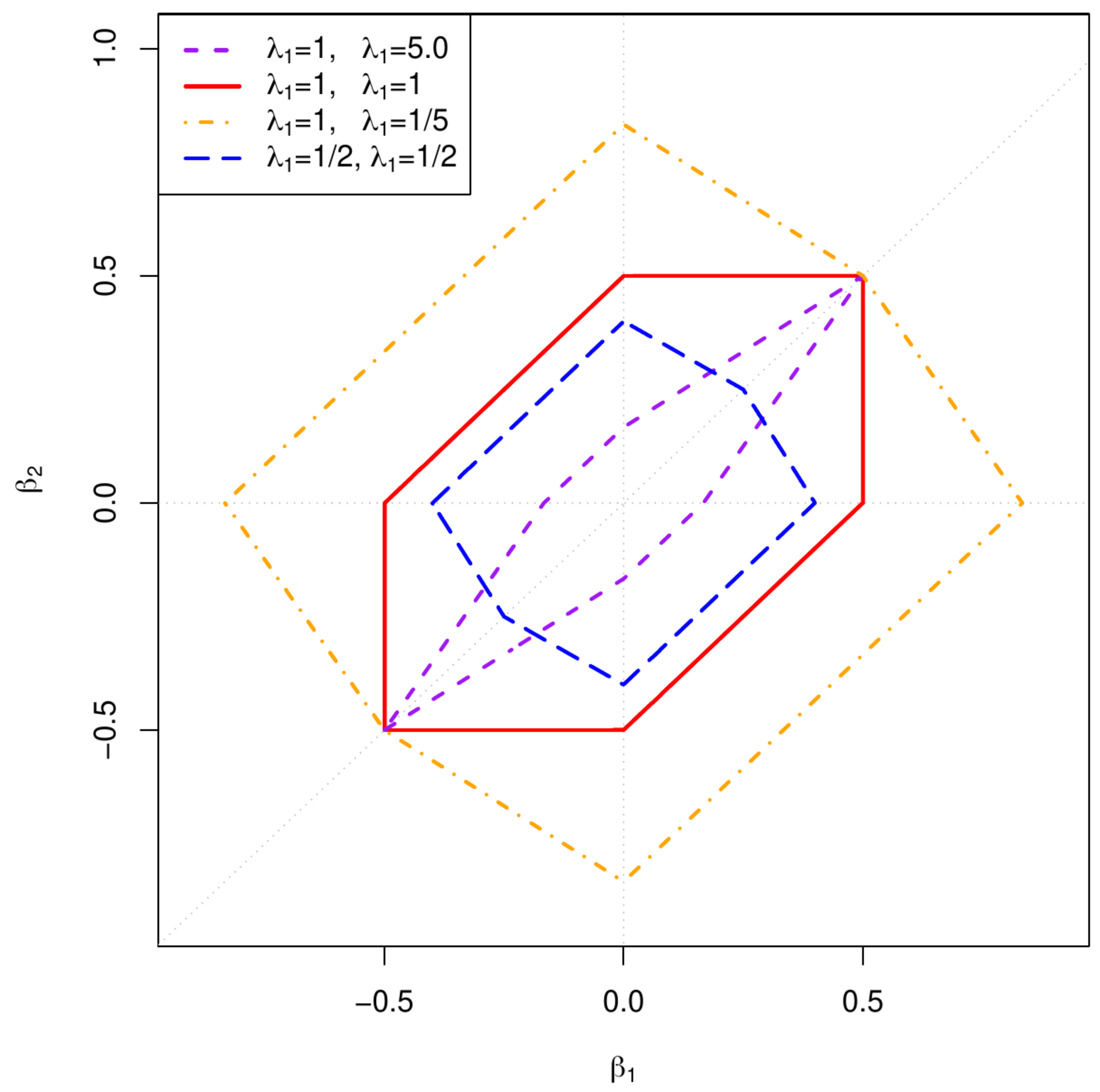
The left panel shows the lasso (red, diamonds) and fused lasso (black circles) regression parameter estimates and the true parameter values (grey circles) plotted against their index [math]j[/math]. The [math](\beta_1, \beta_2)[/math]-parameter constraint induced by the fused lasso penalty for various combinations of the lasso and fusion penalty parameters [math]\lambda_1[/math] and [math]\lambda_{1,f}[/math], respectively. The grey dotted lines corresponds to the ‘[math]\beta_1 = 0[/math]’-, ‘[math]\beta_2 = 0[/math]’- and ‘[math]\beta_1 = \beta_2[/math]’-lines where selection takes place.

It is insightful to view the fused lasso regression problem as a constrained estimation problem. The fused lasso penalty induces a parameter constraint: [math]\{ \bbeta \in \mathbb{R}^p \, : \, \lambda_1 \| \bbeta \|_1 + \lambda_{1,f} \sum_{j=2}^p | \beta_{j} - \beta_{j-1} | \leq c(\lambda_1, \lambda_{1,f}) \}[/math]. This constraint is plotted for [math]p=2[/math] in the right panel of Figure (clearly, it is not the intersection of the constraints induced by the lasso and fusion penalty separately as one might accidently conclude from Figure 2 in ). The constraint is convex, although not strict, which is convenient for optimization purposes. Morever, the geometry of this fused lasso constraint reveals why the fused lasso regression estimator selects the elements of [math]\bbeta[/math] as well as its first order difference. Its boundary, while continuous and generally smooth, has six points at which it is non-differentiable. These all fall on the grey dotted lines in the right panel of Figure that correspond to the axes and the diagonal, put differently, on either the ‘[math]\beta_1 = 0[/math]’, ‘[math]\beta_2 = 0[/math]’ , or ‘[math]\beta_1 = \beta_2[/math]’-lines. The fused lasso regression estimate is the point where the smallest level set of the sum-of-squares criterion [math]\| \mathbf{Y} - \mathbf{X} \bbeta \|_2^2[/math], be it an ellipsoid or hyper-plane, hits the fused lasso constraint. For an element or the first order difference to be zero it must fall on one of the dotted greys lines of the right panel of Figure. Exactly this happens on one of the aforementioned six point of the constraint. Finally, the fused lasso regression estimator has, when -- for reasonably comparable penalty parameters [math]\lambda_1[/math] and [math]\lambda_{1,f}[/math] -- it shrinks the first order difference to zero, a tendency to also estimate the corresponding individual elements as zero. In part, this is due to the fact that [math]| \beta_1 | = 0 = | \beta_2|[/math] implies that [math]| \beta_1 - \beta_2 | = 0[/math], while the reverse does not necessary hold. Moreover, if [math]|\beta_1| = 0[/math], then [math]|\beta_1 - \beta_2|= | \beta_2|[/math]. The fusion penalty thus converts to a lasso penalty of the remaining nonzero element of this first order difference, i.e. [math](\lambda_1 + \lambda_{1,f}) | \beta_2|[/math], thus furthering the shrinkage of this element to zero.

The evaluation of the fused lasso regression estimator is more complicated than that of the ‘ordinary’ lasso regression estimator. For ‘moderately sized’ problems suggest to use a variant of the quadratic programming method (see also Section Quadratic programming ) that is computationally efficient when many linear constraints are active, i.e. when many elements of and first order difference of [math]\bbeta[/math] are zero. extend the gradient ascent approach discussed in Section Gradient ascent to solve the minimization of the fused lasso loss function. For the limiting ‘[math]\lambda_1=0[/math]’-case the fused lasso loss function can be reformulated as a lasso loss function (see Exercise). Then, the algorithms of Section Estimation may be applied to find the estimate [math]\hat{\bbeta} (0, \lambda_{1,f})[/math].

The (sparse) group lasso

The lasso regression estimator selects covariates, irrespectively of the relation among them. However, groups of covariates may be discerned. For instance, a group of covariates may be dummy variables representing levels of a categorical factor. Or, within the context of gene expression studies such groups may be formed by so-called pathways, i.e. sets of genes that work in concert to fulfill a certain function in the cell. In such cases a group-structure can be overlayed on the covariates and it may be desirable to select the whole group, i.e. all covariates together, rather than an individual covariate of the group. To achieve this proposed the group lasso regression estimator. It minimizes the sum-of-squares now augmented with the group lasso penalty, i.e.:

[[math]] \begin{eqnarray*} \lambda_{1,G} \sum\nolimits_{g = 1}^G \sqrt{|\mathcal{J}_g|} \, \| \bbeta_g \|_2 & = & \lambda_{1,G} \sum\nolimits_{g = 1}^G \sqrt{|\mathcal{J}_g|} \sqrt{\sum\nolimits_{j \in \mathcal{J}_g} \beta_j^2}, \end{eqnarray*} [[/math]]

where [math]\lambda_{1, G}[/math] is the group lasso penalty parameter (with subscript [math]G[/math] for Group), [math]G[/math] is the total number of groups, [math]\mathcal{J}_g \subset \{1, \ldots, p \}[/math] is covariate index set of the [math]g[/math]-th group such that the [math]\mathcal{J}_g[/math] are mutually exclusive and exhaustive, i.e. [math]\mathcal{J}_{g_1} \cap \mathcal{J}_{g_2} = \emptyset[/math] for all [math]g_1 \not= g_2[/math] and [math]\cup_{g=1}^G \mathcal{J}_g = \{1, \ldots, p \}[/math], and [math]|\mathcal{J}_g|[/math] denotes the cardinality (the number of elements) of [math]\mathcal{J}_g[/math].

The group lasso estimator performs covariate selection at the group level but does not result in a sparse within-group estimate. This may be achieved through employment of the sparse group lasso regression estimator :

[[math]] \begin{eqnarray*} \hat{\bbeta}(\lambda_1, \lambda_{1,G}) & = & \arg \min_{\bbeta \in \mathbb{R}^p} \| \mathbf{Y} - \mathbf{X} \bbeta \|_2^2 + \lambda_1 \| \bbeta \|_1 + \lambda_{1,G} \sum\nolimits_{g = 1}^G \sqrt{|J_g|} \, \| \bbeta_g \|_2, \end{eqnarray*} [[/math]]

which combines the lasso with the group lasso penalty. The inclusion of the former encourages within-group sparsity, while the latter performs selection at the group level. The sparse group lasso penalty resembles the elastic net penalty with the [math]\| \bbeta \|_2[/math]-term replacing the [math]\| \bbeta \|_2^2[/math]-term of the latter.

Top left panel: The [math](\beta_1, \beta_2)[/math]-parameter constraint induced by the lasso, group lasso and sparse group lasso penalty.

Top right panel: the adaptive threshold function associated with the adaptive lasso regression estimator for orthonormal design matrices.

Bottom left panel: illustration of the lasso and adaptive lasso fit and the true curve.

Bottom right panel: the parameter constraint induced by the [math]\ell_0[/math]-penalty.

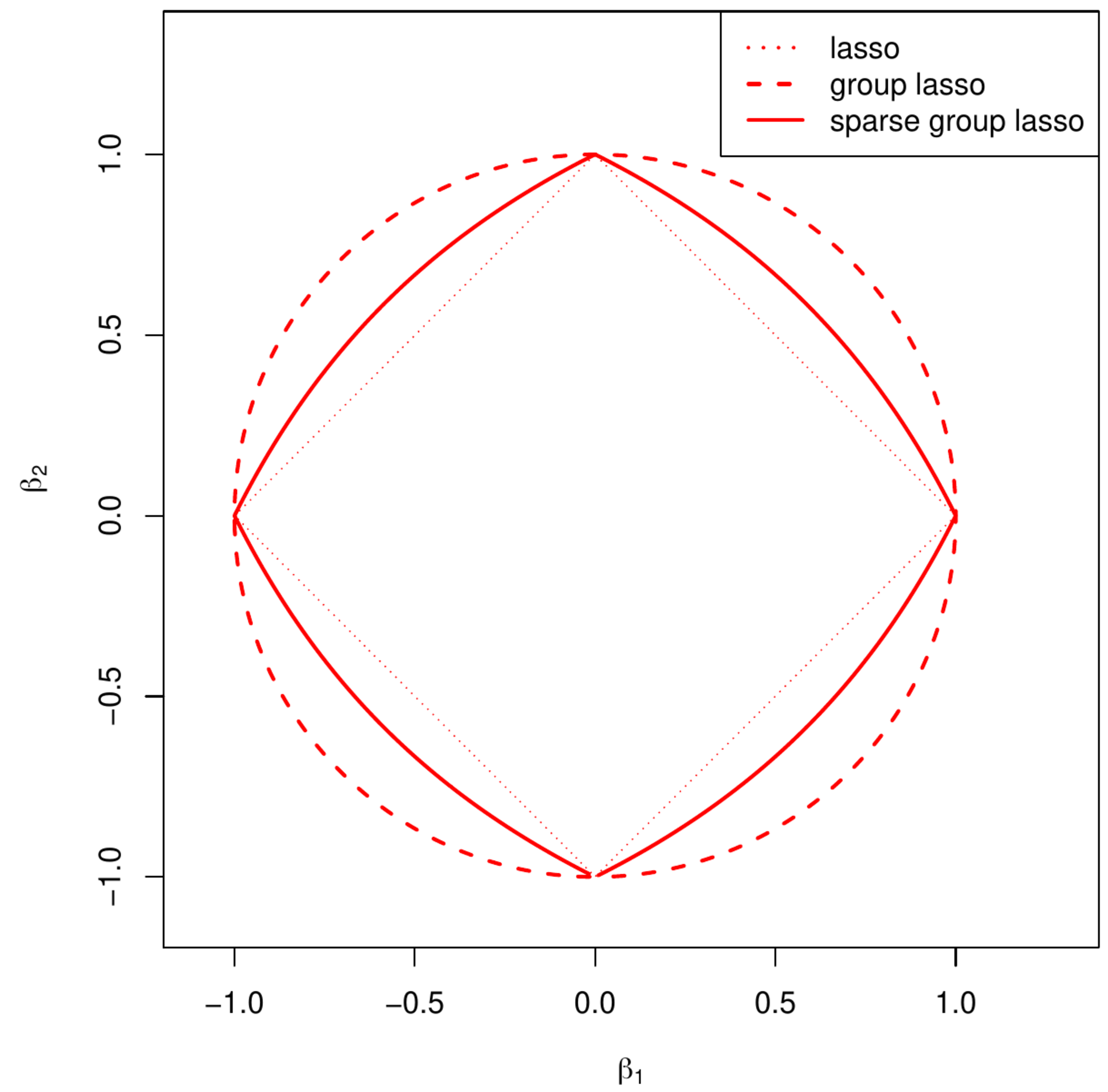
The (sparse) group lasso regression estimation problems can be reformulated as constrained estimation problems. Their parameter constraints are depicted in Figure. By now the reader will be familiar with the charactistic feature, i.e. the non-differentiability of the boundary at the axes, of the constraint that endows the estimator with the potential to select. This feature is clearly present for the sparse group lasso regression estimator, covariate-wise. Although both the group lasso and the sparse group lasso regression estimator select group-wise, illustration of the associated geometrical feature requires plotting in dimensions larger than two and is not attempted. However, when all groups are singletons, the (sparse) group lasso penalties are equivalent to the regular lasso penalty.

The sparse group lasso regression estimator is found through exploitation of the convexity of the loss function . It alternates between group-wise and within-group optimization. The resemblance of the sparse group lasso and elastic net penalties propagates to the optimality conditions of both estimators. In fact, the within-group optimization amounts to the evaluation of an elastic net regression estimator . When within each group the design matrix is orthonormal and [math]\lambda_{1,G} = 0[/math], the group lasso regression estimator can be found by a group-wise coordinate descent procedure for the evaluation of the estimator (cf. Exercise \ref{}).

Both the sparse group lasso and the elastic net regression estimators have two penalty parameters that need tuning. In both cases the corresponding penalties have a similar effect: shrinkage towards zero. If the [math]g[/math]-th group's contribution to the group lasso penalty has vanished, then so has the contribution of all covariates to the regular lasso penalty. And vice versa. This complicates the tuning of the penalty parameters as it is hard to distinguish which shrinkage effect is most beneficial for the estimator. resolve this by setting the ratio of the two penalty parameters [math]\lambda_1[/math] and [math]\lambda_{1,G}[/math] to some arbitrary but fixed value, thereby simplifying the tuning.

Adaptive lasso

The lasso regression estimator does not exhibit some key and desirable asymptotic properties. proposed the \text{adaptive lasso} regression estimator to achieve these properties. The adaptive lasso regression estimator is a two-step estimation procedure. First, an initial estimator of the regression parameter [math]\bbeta[/math], denoted [math]\hat{\bbeta} ^{\mbox{{\tiny init}}}[/math], is to be obtained. The adaptive lasso regression estimator is then defined as:

[[math]] \begin{eqnarray*} \hat{\bbeta}^{\mbox{{\tiny adapt}}} (\lambda_1) & = & \arg \min_{\bbeta \in \mathcal{R}^p} \| \mathbf{Y} - \mathbf{X} \bbeta \|_2^2 + \lambda_1 \sum\nolimits_{j=1}^p | \hat{\beta}^{\mbox{{\tiny init}}}_j |^{-1} | \beta_j |. \end{eqnarray*} [[/math]]

Hence, it is a generalization of the lasso penalty with covariate-specific weighing. The weight of the [math]j[/math]-th covariate is reciprocal to the [math]j[/math]-th element of the initial regression parameter estimate [math]\hat{\bbeta}^{\mbox{{\tiny init}}}[/math]. If the initial estimate of [math]\beta_j[/math] is large or small, the corresponding element in the adaptive lasso estimator will be penalized less or more and thereby determine the amount of shrinkage, which may now vary between the estimates of the elements of [math]\bbeta[/math]. In particular, if [math]\hat{\bbeta}_j^{\mbox{{\tiny init}}} = 0[/math], the adaptive lasso penalty parameter corresponding to the [math]j[/math]-th element is infinite and yields [math]\hat{\bbeta}^{\mbox{{\tiny adapt}}} = 0[/math].

The adaptive lasso regression estimator, given an initial regression estimate [math]\hat{\bbeta}^{\mbox{{\tiny init}}}[/math], can be found numerically by minor changes of the algorithms presented in Section Estimation . In case of an orthonormal design an analytic expression of the adaptive lasso estimator exists (see Exercise):

[[math]] \begin{eqnarray*} \hat{\beta}_j^{\mbox{{\tiny adapt}}} (\lambda_1) & = & \mbox{sign}(\hat{\beta}_j^{\mbox{{\tiny ols}}}) ( | \hat{\beta}_j^{\mbox{{\tiny ols}}} | - \tfrac{1}{2} \lambda_1 / | \hat{\beta}_j^{\mbox{{\tiny ols}}} |)_+. \end{eqnarray*} [[/math]]

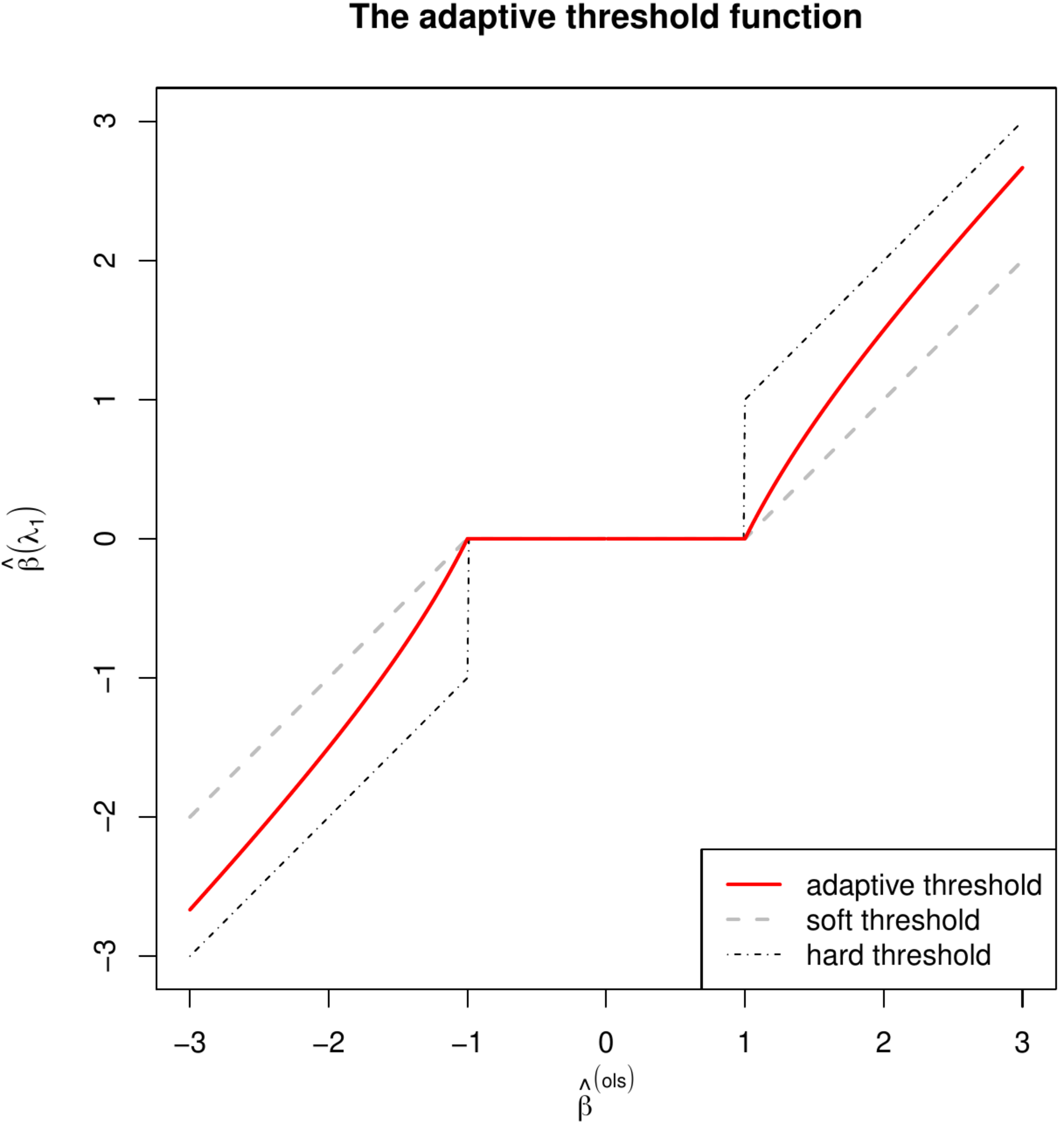
This adaptive lasso estimator can be viewed as a compromise between the soft thresholding function, associated with the lasso regression estimator for orthonormal design matrices (Section Analytic solutions ), and the hard thresholding function, associated with truncation of the ML regression estimator (see the top right panel of Figure for an illustration of these thresholding functions).

How is the initial regression parameter estimate [math]\hat{\bbeta}^{\mbox{{\tiny init}}}[/math] to be chosen? Low-dimensionally the maximum likelihood regression estimator one may used. The resulting adaptive lasso regression estimator is sometimes referred to as the Gauss-Lasso regression estimator. High-dimensionally, the lasso or ridge regression estimators will do. Any other estimator may in principle be used. But not all yield the desirable asymptotic properties.

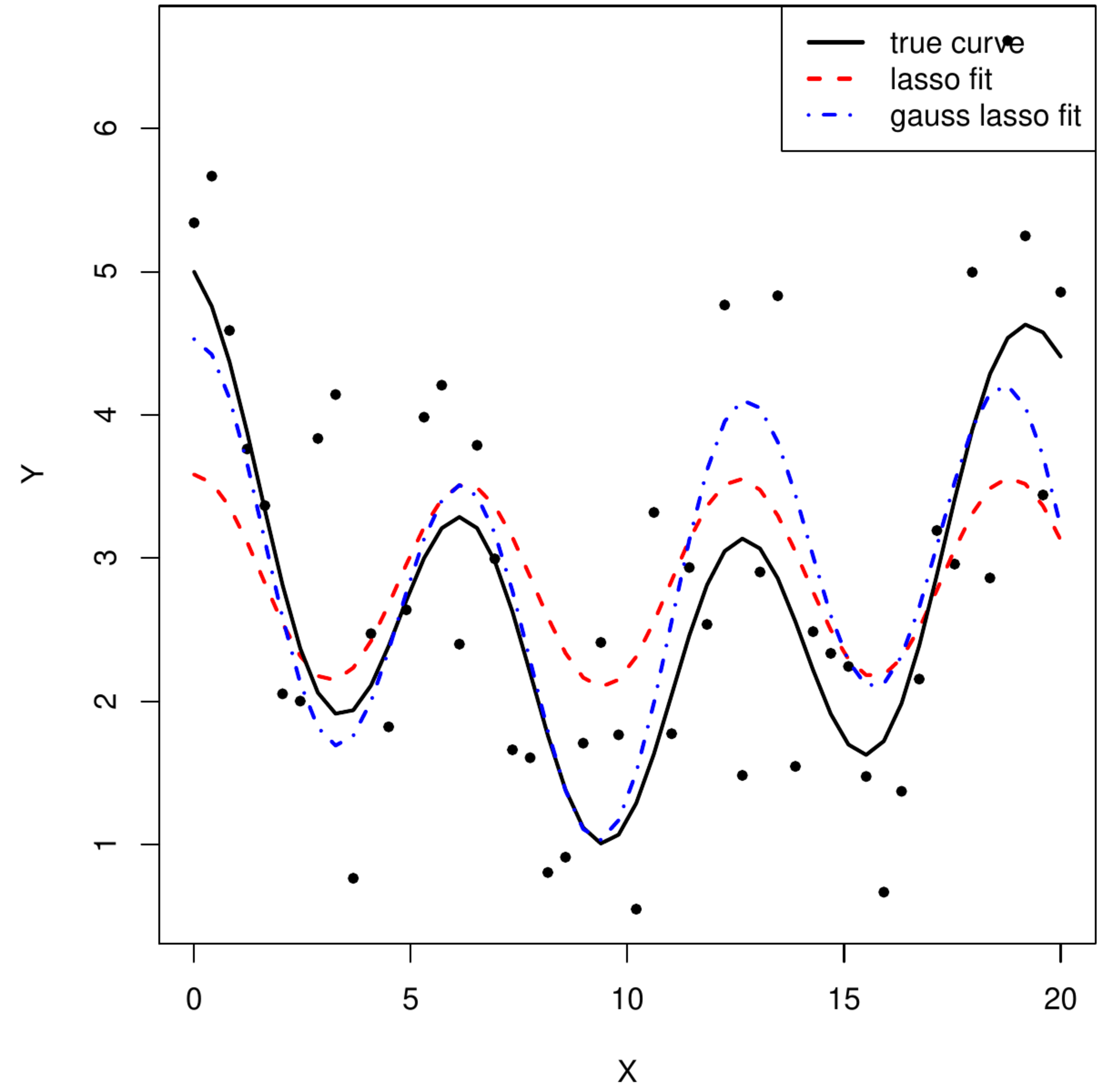
A different motivation for the adaptive lasso is found in its ability to undo some or all of the shrinkage of the lasso regression estimator due to penalization. This is illustrated in the left bottom panel of Figure. It shows the lasso and adaptive lasso regression fits. The latter clearly undoes some of the bias of the former.

The [math]\ell_0[/math] penalty

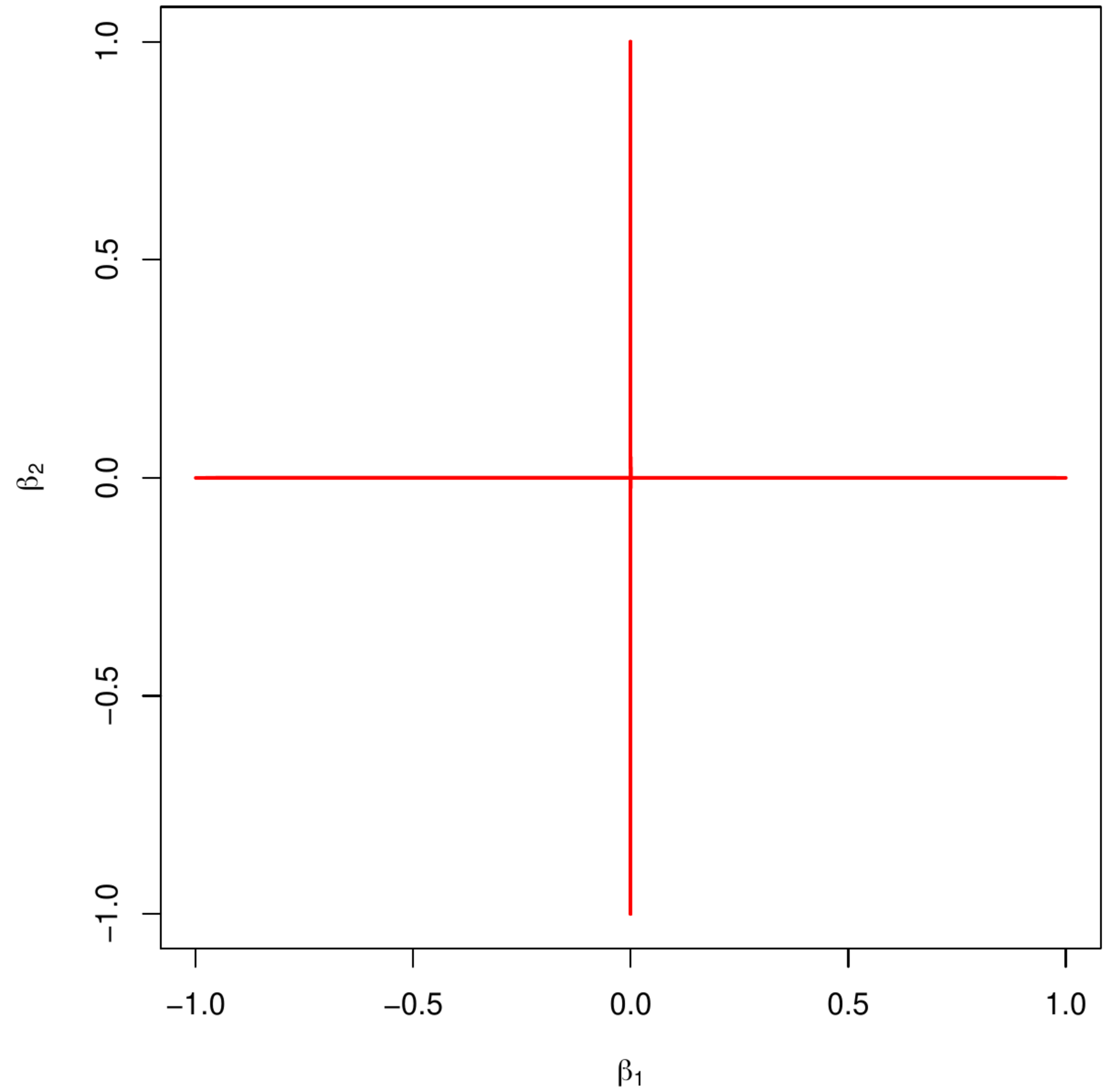
An alternative estimators, considered to be superior to both the lasso and ridge regression estimators, is the [math]\ell_0[/math]-penalized regression estimator. It too minimizes the sum-of-squares now with the [math]\ell_0[/math]-penalty. The [math]\ell_0[/math]-penalty, denoted [math]\lambda_0 \| \bbeta \|_0[/math], is defined as [math]\lambda_0 \| \bbeta \|_0 = \lambda_0 \sum_{j=1}^p I_{ \{ \beta_j \not= 0 \} }[/math] with penalty parameter [math]\lambda_0[/math] and [math]I_{\{ \cdot \}}[/math] the indicator function. The parameter constraint associated with this penalty is shown in the right panel of Figure. From the form of the penalty it is clear that the [math]\ell_0[/math]-penalty penalizes only for the presence of a covariate in the model. As such it is concerned with the number of covariates in the model, and not the size of their regression coefficients (or a derived quantity thereof). The latter is considered only a surrogate of the number of covariates in the model. As such the lasso and ridge estimators are proxies to the [math]\ell_0[/math]-penalized regression estimator.

The [math]\ell_0[/math]-penalized regression estimator is not used for large dimensional problems as its evaluation is computationally too demanding. It requires a search over all possible subsets of the [math]p[/math] covariates to find the optimal model. As each covariate can either be in or out of the model, in total [math]2^p[/math] models need to be considered. This is not feasible with present-day computers.

The adaptive lasso regression estimator may be viewed as an approximation of the [math]\ell_0[/math]-penalized regression estimator. When the covariate-wise weighing employed in the penalization of the adaptive lasso regression estimation is equal to [math]\lambda_{1,j} = \lambda / |\beta_j|[/math] with [math]\beta_j[/math] known true value of the [math]j[/math]-th regression coefficient, the [math]j[/math]-th covariate's estimated regression coefficient contributes only to the penalty if it is nonzero. In practice, this weighing involves an initial estimate of [math]\bbeta[/math] and is therefore an approximation at best, which the quality of the approximation hinging upon that of the weighing.

General References

van Wieringen, Wessel N. (2021). "Lecture notes on ridge regression". arXiv:1509.09169 [stat.ME].

References

- 1.0 1.1 Zou, H. and Hastie, T. (2005).Regularization and variable selection via the elastic net.Journal of the Royal Statistical Society: Series B (Statistical Methodology), 67(2), 301--320
- Friedman, J., Hastie, T., and Tibshirani, R. (2009).glmnet: Lasso and elastic-net regularized generalized linear models.R package version, 1(4)
- 3.0 3.1 3.2 Tibshirani, R., Saunders, M., Rosset, S., Zhu, J., and Knight, K. (2005).Sparsity and smoothness via the fused lasso.Journal of the Royal Statistical Society: Series B (Statistical Methodology), 67(1), 91--108
- Chaturvedi, N., de Menezes, R. X., and Goeman, J. J. (2014).Fused lasso algorithm for Cox' proportional hazards and binomial logit models with application to copy number profiles.Biometrical Journal, 56(3), 477--492
- Yuan, M. and Lin, Y. (2006).Model selection and estimation in regression with grouped variables.Journal of the Royal Statistical Society: Series B (Statistical Methodology), 68(1), 49--67
- 6.0 6.1 6.2 6.3 Simon, N., Friedman, J., Hastie, T., and Tibshirani, R. (2013).A sparse-group lasso.Journal of Computational and Graphical Statistics, 22(2), 231--245
- Zou, H. (2006).The adaptive lasso and its oracle properties.Journal of the American Statistical Association, 101(476), 1418--1429