Lasso Regression
[math] \require{textmacros} \def \bbeta {\bf \beta} \def\fat#1{\mbox{\boldmath$#1$}} \def\reminder#1{\marginpar{\rule[0pt]{1mm}{11pt}}\textbf{#1}} \def\SSigma{\bf \Sigma} \def\ttheta{\bf \theta} \def\aalpha{\bf \alpha} \def\bbeta{\bf \beta} \def\ddelta{\bf \delta} \def\eeta{\bf \eta} \def\llambda{\bf \lambda} \def\ggamma{\bf \gamma} \def\nnu{\bf \nu} \def\vvarepsilon{\bf \varepsilon} \def\mmu{\bf \mu} \def\nnu{\bf \nu} \def\ttau{\bf \tau} \def\SSigma{\bf \Sigma} \def\TTheta{\bf \Theta} \def\XXi{\bf \Xi} \def\PPi{\bf \Pi} \def\GGamma{\bf \Gamma} \def\DDelta{\bf \Delta} \def\ssigma{\bf \sigma} \def\UUpsilon{\bf \Upsilon} \def\PPsi{\bf \Psi} \def\PPhi{\bf \Phi} \def\LLambda{\bf \Lambda} \def\OOmega{\bf \Omega} [/math]
We return to the linear regression model, which is still fitted in penalized fashion but this time with a so-called lasso penalty. Yet another penalty? Yes, but the resulting estimator will turn out to have interesting properties. The outline of this chapter loosely follows that of its counterpart on ridge regression.
Recall that ridge regression finds an estimator of the parameter of the linear regression model through the minimization of:
with [math]f_{\mbox{{\scriptsize pen}}}(\bbeta, \lambda) = \lambda \| \bbeta \|_2^2[/math]. The particular choice of the penalty function originated in a post-hoc motivation of the ad-hoc fix to the singularity of the matrix [math]\mathbf{X}^{\top} \mathbf{X}[/math], stemming from the design matrix [math]\mathbf{X}[/math] not being of full rank (i.e. [math]\mbox{rank}(\mathbf{X}) \lt p[/math]). The ad-hoc nature of the fix suggests that the choice for the squared Euclidean norm of [math]\bbeta[/math] as a penalty is arbitrary and other choices may be considered, some of which were already encountered in Chapter Generalizing ridge regression .
One such choice is the so-called lasso penalty, giving rise to lasso regression, as introduced by [1]. Like ridge regression, lasso regression fits the linear regression model [math]\mathbf{Y} = \mathbf{X} \bbeta + \vvarepsilon[/math] with the standard assumption on the error [math]\vvarepsilon[/math]. Like ridge regression, it does so by minimization of the sum of squares augmented with a penalty. Hence, lasso regression too minimizes loss function (\ref{form.penLeastSquares}). The difference with ridge regression is in the penalty function. Instead of the squared Euclidean norm, lasso regression uses the [math]\ell_1[/math]-norm: [math]f_{\mbox{{\scriptsize pen}}}(\bbeta, \lambda_1) = \lambda_1 \| \bbeta \|_1[/math], the sum of the absolute values of the regression parameters multiplied by the lasso penalty parameter [math]\lambda_1[/math]. To distinguish the ridge and lasso penalty parameters, they are henceforth denoted [math]\lambda_2[/math] and [math]\lambda_1[/math], respectively, with the subscript referring to the norm used in the penalty. The lasso regression loss function is thus:
The lasso regression estimator is then defined as the minimizer of this loss function. As with the ridge regression loss function, the maximum likelihood estimator (should it exists) of [math]\bbeta[/math] minimizes the first part, while the second part is minimized by setting [math]\bbeta[/math] equal to the [math]p[/math] dimensional zero vector. For [math]\lambda_1[/math] close to zero, the lasso estimate is close to the maximum likelihood estimate. Whereas for large [math]\lambda_1[/math], the penalty term overshadows the sum-of-squares, and the lasso estimate is small (in some sense). Intermediate choices of [math]\lambda_1[/math] mold a compromise between those two extremes, with the penalty parameter determining the contribution of each part to this compromise. The lasso regression estimator thus is not one but a whole sequence of estimators of [math]\bbeta[/math], one for every [math]\lambda_1 \in \mathbb{R}_{\gt0}[/math]. This sequence is the lasso regularization path, defined as [math]\{ \hat{\bbeta}(\lambda_1) \, : \, \lambda_1 \in \mathbb{R}_{\gt0} \}[/math]. To arrive at a final lasso estimator of [math]\bbeta[/math], like its ridge counterpart, the lasso penalty parameter [math]\lambda_1[/math] needs to be chosen (see Section \ref{sect:lassoPenaltyChoice}).
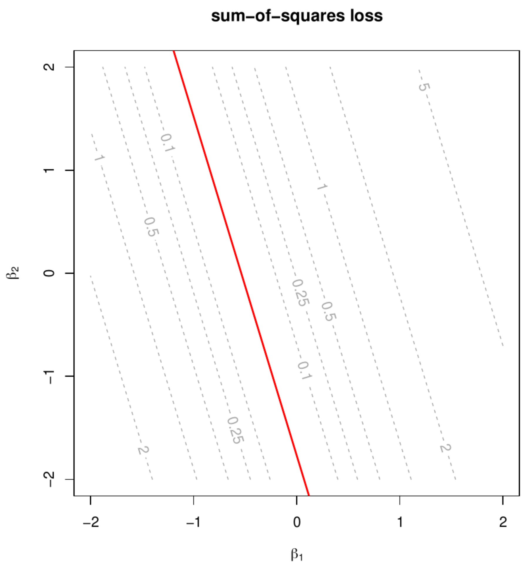
Contour plots of the sum-of-squares and the lasso regression loss (left and right panel, respectively). The dotted grey line represent level sets. The red line and dot represent the location of minimum in both panels.
The [math]\ell_1[/math] penalty of lasso regression is equally arbitrary as the [math]\ell_2^2[/math]-penalty of ridge regression. The latter ensured the existence of a well-defined estimator of the regression parameter [math]\bbeta[/math] in the presence of super-collinearity in the design matrix [math]\mathbf{X}[/math], in particular when the dimension [math]p[/math] exceeds the sample size [math]n[/math]. The augmentation of the sum-of-squares with the lasso penalty achieves the same. This is illustrated in Figure. For the high-dimensional setting with [math]p=2[/math] and [math]n=1[/math] and arbitrary data the level sets of the sum-of-squares [math]\| \mathbf{Y} - \mathbf{X} \, \bbeta \|^2_2[/math] and the lasso regression loss [math]\| \mathbf{Y} - \mathbf{X} \, \bbeta \|^2_2 + \lambda_1 \| \bbeta \|_1[/math] are plotted (left and right panel, respectively). In both panels the minimum is indicated in red. For the sum-of-squares the minimum is a line. As pointed out before in Section The ridge regression estimator of Chapter Ridge regression on ridge regression, this minimum is determined up to an element of the null set of the design matrix [math]\mathbf{X}[/math], which in this case is non-trivial. In contrast, the lasso regression loss exhibits a unique well-defined minimum. Hence, the augmentation of the sum-of-squares with the lasso penalty yields a well-defined estimator of the regression parameter. (This needs some attenuation: in general the minimum of the lasso regression loss need not be unique, confer Section Uniqueness ).
The mathematics involved in the derivation in this chapter tends to be more intricate than for ridge regression. This is due to the non-differentiability of the lasso penalty at zero. This has consequences on all aspects of the lasso regression estimator as is already obvious in the right-hand panel of Figure: confer the non-differentiable points of the lasso regression loss level sets.
Uniqueness
The lasso regression loss function is the sum of the sum-of-squares criterion and a sum of absolute value functions. Both are convex in [math]\bbeta[/math]: the former is not strict convex due to the high-dimensionality and the absolute value function is convex due to its piece-wise linearity. Thereby the lasso loss function too is convex but not strict. Consequently, its minimum need not be uniquely defined. But, the set of solutions of a convex minimization problem is convex (Theorem 9.4.1, Fletcher, 1987). Hence, would there exist multiple minimizers of the lasso loss function, they can be used to construct a convex set of minimizers. Thus, if [math]\hat{\bbeta}_a (\lambda_1)[/math] and [math]\hat{\bbeta}_b (\lambda_1)[/math] are lasso estimators, then so are [math](1-\theta) \hat{\bbeta}_a (\lambda_1) + \theta \hat{\bbeta}_b (\lambda_1)[/math] for [math]\theta \in (0,1)[/math]. This is illustrated in Example.
Example (Perfectly super-collinear covariates)
Consider the standard linear regression model [math]Y_i = \mathbf{X}_{i,\ast} \bbeta + \varepsilon_i[/math] for [math]i=1, \ldots, n[/math] and with the [math]\varepsilon_i[/math] i.i.d. normally distributed with zero mean and a common variance. The rows of the design matrix [math]\mathbf{X}[/math] are of length two, neither column represents the intercept, but [math]\mathbf{X}_{\ast, 1} = \mathbf{X}_{\ast, 2}[/math]. Suppose an estimate of the regression parameter [math]\bbeta[/math] of this model is obtained through the minimization of the sum-of-squares augmented with a lasso penalty, [math]\| \mathbf{Y} - \mathbf{X} \bbeta \|_2^2 + \lambda_1 \| \bbeta \|_1[/math] with penalty parameter [math]\lambda_1 \gt 0[/math]. To find the minimizer define [math]u = \beta_1 + \beta_2[/math] and [math]v = \beta_1 - \beta_2[/math] and rewrite the lasso loss criterion to:
The function [math]| u + v |+ | u - v |[/math] is minimized with respect to [math]v[/math] for any [math]v[/math] such that [math]|v| \lt |u|[/math] and the corresponding minimum equals [math]2| u|[/math]. The estimator of [math]u[/math] thus minimizes:
For sufficiently small values of [math]\lambda_1[/math] the estimate of [math]u[/math] will be unequal to zero. Then, any [math]v[/math] such that [math]|v| \lt |u|[/math] will yield the same minimum of the lasso loss function. Consequently, [math]\hat{\bbeta}(\lambda_1)[/math] is not uniquely defined as [math]\hat{\beta}_1(\lambda_1) = \tfrac{1}{2} [\hat{u}(\lambda_1) + \hat{v}(\lambda_1)][/math] need not equal [math]\hat{\beta}_2(\lambda_1) = \tfrac{1}{2} [\hat{u}(\lambda_1) - \hat{v}(\lambda_1)][/math] for any [math]\hat{v}(\lambda_1)[/math] such that [math]0 \lt | \hat{v}(\lambda_1) | \lt |\hat{u}(\lambda_1)|[/math].
The lasso regression estimator [math]\hat{\bbeta}(\lambda_1)[/math] need not be unique, but its linear predictor [math]\mathbf{X} \hat{\bbeta}(\lambda_1)[/math] is. This can be proven by contradiction [2]. Suppose there exists two lasso regression estimators of [math]\bbeta[/math], denoted [math]\hat{\bbeta}_a (\lambda_1)[/math] and [math]\hat{\bbeta}_b (\lambda_1)[/math], such that [math]\mathbf{X} \hat{\bbeta}_a (\lambda_1) \not= \mathbf{X} \hat{\bbeta}_b (\lambda_1)[/math]. Define [math]c[/math] to be the minimum of the lasso loss function. Then, by definition of the lasso estimators [math]\hat{\bbeta}_a (\lambda_1)[/math] and [math]\hat{\bbeta}_b (\lambda_1)[/math] satisfy:
For [math]\theta \in (0,1)[/math] we then have:
by the strict convexity of [math]\| \mathbf{Y} - \mathbf{X} \bbeta \|_2^2[/math] in [math]\mathbf{X} \bbeta[/math] and the convexity of [math]\| \bbeta \|_1[/math] on [math]\theta \in (0,1)[/math]. This implies that [math](1-\theta) \hat{\bbeta}_a (\lambda_1) + \theta \hat{\bbeta}_b (\lambda_1)[/math] yields a lower minimum of the lasso loss function and contradicts our assumption that [math]\hat{\bbeta}_a (\lambda_1)[/math] and [math]\hat{\bbeta}_b (\lambda_1)[/math] are lasso regression estimators. Hence, the lasso linear predictor is unique.
Example (Perfectly super-collinear covariates, revisited)
Revisit the setting of Example, where a linear regression model without intercept and only two but perfectly correlated covariates is fitted to data. The example revealed that the lasso estimator need not be unique. The lasso predictor, however, is
with [math]u[/math] defined and (uniquely) estimated as in Example and [math]v[/math] dropping from the predictor.
Analytic solutions
In general, no explicit expression for the lasso regression estimator exists. There are exceptions, as illustrated in Examples example.orthonormalDesignLasso and example:lassoPequals. Nonetheless, it is possible to show properties of the lasso estimator, amongst others of the smoothness of its regularization path (Theorem) and the limiting behaviour as [math]\lambda_1 \rightarrow \infty[/math] (see the end of this section).
The lasso regression loss function (\ref{form.lassoLossFunction}) yields a piecewise linear, in [math]\lambda_1[/math], regularization path [math]\{ \hat{\bbeta}(\lambda_1) : \mathbb{R}_{\gt0} \}[/math].
Show Proof
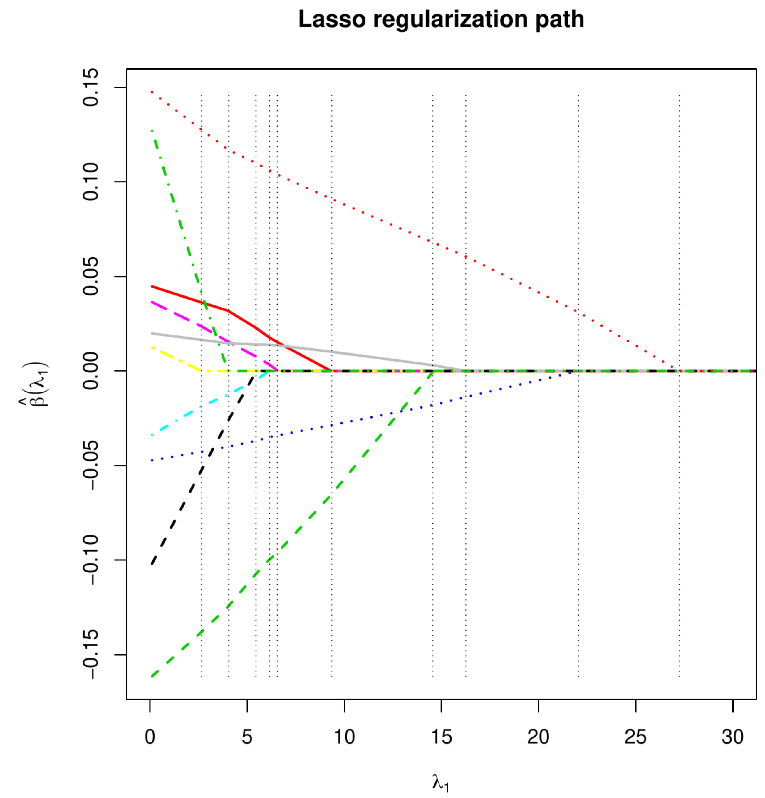
This piecewise linear nature of the lasso solution path is illustrated in the left-hand panel of Figure of an arbitrary data set. At each vertical dotted line a discontinuity in the derivative with respect to [math]\lambda_1[/math] of the regularization path of a lasso estimate of an element of [math]\bbeta[/math] may occur. The plot also foreshadows the [math]\lambda_1 \rightarrow \infty[/math] limiting behaviour of the lasso regression estimator: the estimator tends to zero. This is no surprise knowing that the ridge regression estimator exhibits the same behaviour and the lasso regression loss function is of similar form as that of ridge regression: a sum-of-squares plus a penalty term (which is linear in the penalty parameter).
The left panel shows the regularization path of the lasso regression estimator for simulated data. The vertical grey dotted lines indicate the values of [math]\lambda_1[/math] at which there is a discontinuity in the derivative (with respect to [math]\lambda_1[/math]) of the lasso regularization path of one the regression estimates. The right panel displays the soft (solid, red) and hard (grey, dotted) threshold functions.
For particular cases, an orthormal design (Example) and [math]p=2[/math] (Example), an analytic expression for the lasso regression estimator exists. While the latter is of limited use, the former is exemplary and will come of use later in the numerical evaluation of the lasso regression estimator in the general case (see Section Estimation ).
Example (Orthonormal design matrix)
Consider an orthonormal design matrix [math]\mathbf{X}[/math], i.e. [math]\mathbf{X}^{\top} \mathbf{X} = \mathbf{I}_{pp} = (\mathbf{X}^{\top} \mathbf{X})^{-1}[/math]. The lasso estimator then is:
where [math]\hat{\bbeta} = (\mathbf{X}^{\top} \mathbf{X})^{-1} \mathbf{X}^{\top} \mathbf{Y} = \mathbf{X}^{\top} \mathbf{Y}[/math] is the maximum likelihood estimator of [math]\bbeta[/math] and [math]\hat{\beta}_j[/math] its [math]j[/math]-th element and [math]f(x) = (x)_+ = max\{x, 0\}[/math]. This expression for the lasso regression estimator can be obtained as follows. Rewrite the lasso regression loss criterion:
The minimization problem can thus be solved per regression coefficient. This gives:
The minimization within the sum over the covariates is with respect to each element of the regression parameter separately. Optimization with respect to the [math]j[/math]-th one gives:
This case-wse solution can be compressed to the form of the lasso regression estimator above.
The analytic expression for the lasso regression estimator above provides insight in how it relates to the maximum likelihood estimator of [math]\bbeta[/math]. The right-hand side panel of Figure depicts this relationship. Effectively, the lasso regression estimator thresholds (after a translation) its maximum likelihood counterpart. The function is also referred to as the soft-threshold function (for contrast the hard-threshold function is also plotted -- dotted line -- in Figure).
Example (Orthogonal design matrix)
The analytic solution of the lasso regression estimator for experiments with an orthonormal design matrix applies to those with an orthogonal design matrix. This is illustrated by a numerical example. Use the lasso estimator with [math]\lambda_1=10[/math] to fit the linear regression model to the response data and the design matrix:
Note that the design matrix is orthogonal, i.e. its columns are orthogonal (but not normalized to one). The orthogonality of [math]\mathbf{X}[/math] yields a diagonal [math]\mathbf{X}^{\top} \mathbf{X}[/math], and so is its inverse [math](\mathbf{X}^{\top} \mathbf{X})^{-1}[/math]. Here [math]\mbox{diag}(\mathbf{X}^{\top} \mathbf{X}) = (22, 28)[/math]. Rescale [math]\mathbf{X}[/math] to an orthonormal design matrix, denoted [math]\tilde{\mathbf{X}}[/math], and rewrite the lasso regression loss function to:
where [math]\ggamma = (\sqrt{22} \beta_1, \sqrt{28} \beta_2)^{\top}[/math]. By the same argument this loss can be minimized with respect to each element of [math]\ggamma[/math] separately. In particular, the soft-threshold function provides an analytic expression for the estimates of [math]\ggamma[/math]:
where [math]\hat{\gamma}_1[/math] and [math]\hat{\gamma}_2[/math] are the ordinary least square estimates of [math]\gamma_1[/math] and [math]\gamma_2[/math] obtained from regressing [math]\mathbf{Y}[/math] on the corresponding column of [math]\tilde{\mathbf{X}}[/math]. Rescale back and obtain the lasso regression estimate: [math]\hat{\bbeta}(10) = (-1.881818, 0.8678572)^{\top}[/math].
Example ([math]p=2[/math] with equivariant covariates, [4])
Let [math]p=2[/math] and suppose the design matrix [math]\mathbf{X}[/math] has equivariant covariates. Without loss of generality they are assumed to have unit variance. We may thus write
for some [math]\rho \in (-1, 1)[/math]. The lasso regression estimator is then of similar form as in the orthonormal case but the soft-threshold function now depends on [math]\lambda_1[/math], [math]\rho[/math] and the maximum likelihood estimate [math]\hat{\bbeta}[/math] (see Exercise).
Apart from the specific cases outlined in the two examples above no other explicit solution for the minimizer of the lasso regression loss function appears to be known. Locally though, for large enough values of [math]\lambda_1[/math], an analytic expression for solution can also be derived. Hereto we point out that (details to be included later) the lasso regression estimator satisfies the following estimating equation:
for some [math]\hat{\mathbf{z}} \in \mathbb{R}^p[/math] with [math](\hat{\mathbf{z}})_j = \mbox{sign}\{[\hat{\bbeta}(\lambda_1)]_j\}[/math] whenever [math][\hat{\bbeta}_j(\lambda_1)]_j \not= 0[/math] and [math](\hat{\mathbf{z}})_j \in [-1,1][/math] if [math][\hat{\bbeta}_j(\lambda_1)]_j = 0[/math]. Then:
For [math]\lambda_1 \gt 2 \| \mathbf{X}^{\top} \mathbf{Y} \|_{\infty}[/math] the summands on the right-hand side satisfy:
This implies that [math]\hat{\bbeta} (\lambda_1) = \mathbf{0}_p[/math] if [math]\lambda_1 \gt 2 \| \mathbf{X}^{\top} \mathbf{Y} \|_{\infty}[/math], where [math]\| \mathbf{a} \|_{\infty}[/math] is the supremum norm of vector [math]\mathbf{a}[/math] defined as [math]\| \mathbf{a} \|_{\infty} = \max \{ |a_1|, |a_2|, \ldots, |a_p | \}[/math].
Sparsity
The change from the [math]\ell_2^2[/math]-norm to the [math]\ell_1[/math]-norm in the penalty may seem only a detail. Indeed, both ridge and lasso regression fit the same linear regression model. But the attractiveness of the lasso lies not in what it fits, but in a consequence of how it fits the linear regression model. The lasso estimator of the vector of regression parameters may contain some or many zero's. In contrast, ridge regression yields an estimator of [math]\bbeta[/math] with elements (possibly) close to zero, but unlikely to be equal to zero. Hence, lasso penalization results in [math]\hat{\beta}_j (\lambda_1) = 0[/math] for some [math]j[/math] (in particular for large values of [math]\lambda_1[/math], see Section Uniqueness ), while ridge penalization yields an estimate of the [math]j[/math]-th element of the regression parameter [math]\hat{\beta}_j (\lambda_2) \not= 0[/math]. A zero estimate of a regression coefficient means that the corresponding covariate has no effect on the response and can be excluded from the model. Effectively, this amounts to variable selection. Where traditionally the linear regression model is fitted by means of maximum likelihood followed by a testing step to weed out the covariates with effects indistinguishable from zero, lasso regression is a one-step-go procedure that simulatenously estimates and selects.
The in-built variable selection of the lasso regression estimator is a geometric accident. To understand how it comes about the lasso regression loss optimization problem (\ref{form.lassoLossFunction}) is reformulated as a constrained estimation problem (using the same argumentation as previously employed for ridge regression, see Section Constrained estimation ):
where [math]c(\lambda_1) = \| \hat{\bbeta}(\lambda_1)\|_1[/math]. Again, this is the standard least squares problem, with the only difference that the sum of the (absolute value of the) regression parameters [math]\beta_1, \beta_2, \ldots, \beta_p[/math] is required to be smaller than [math]c(\lambda_1)[/math]. The effect of this requirement is that the lasso estimator of the regression parameter coefficients can no longer assume any value (from [math]-\infty[/math] to [math]\infty[/math], as is the case in standard linear regression), but are limited to a certain range of values. With the lasso and ridge regression estimators minimizing the same sum-of-squares, the key difference with the constrained estimation formulation of ridge regression is not in the explicit form of [math]c(\lambda_1)[/math] (and is set to some arbitrary convenient value in the remainder of this section) but in what is bounded by [math]c(\lambda_1)[/math] and the domain of acceptable values for [math]\bbeta[/math] that it implies. For the lasso regression estimator the domain is specified by a bound on the [math]\ell_1[/math]-norm of the regression parameter while for its ridge counterpart the bound is applied to the squared [math]\ell_2[/math]-norm of [math]\bbeta[/math]. The parameter constraints implied by the lasso and ridge norms result in balls in different norms:
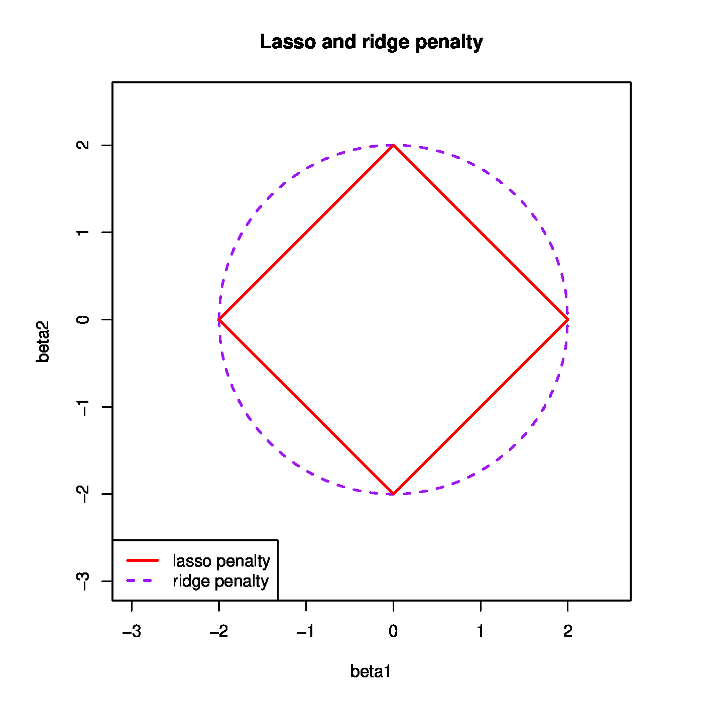
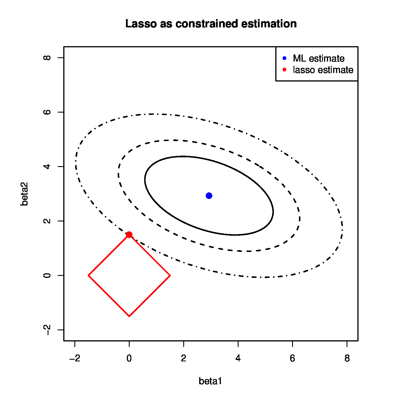
respectively, and where [math]c(\cdot)[/math] is now equipped with a subscript referring to the norm to stress that it is different for lasso and ridge. The left-hand panel of Figure visualizes these parameter constraints for [math]p=2[/math] and [math]c_1(\lambda_1) = 2 = c_2(\lambda_2)[/math]. In the Euclidean space ridge yields a spherical constraint for [math]\bbeta[/math], while a diamond-like shape for the lasso. The lasso regression estimator is then that [math]\bbeta[/math] inside this diamond domain which yields the smallest sum-of-squares (as is visualized by right-hand panel of Figure).
Left panel: The lasso parameter constraint ([math]|\beta_1| + |\beta_2| \leq 2[/math]) and its ridge counterpart ([math]\beta_1^2 + \beta_2^2 \leq 2[/math]). Solution path of the ridge estimator and its variance. Right panel: the lasso regression estimator as a constrained least squares estimtor.
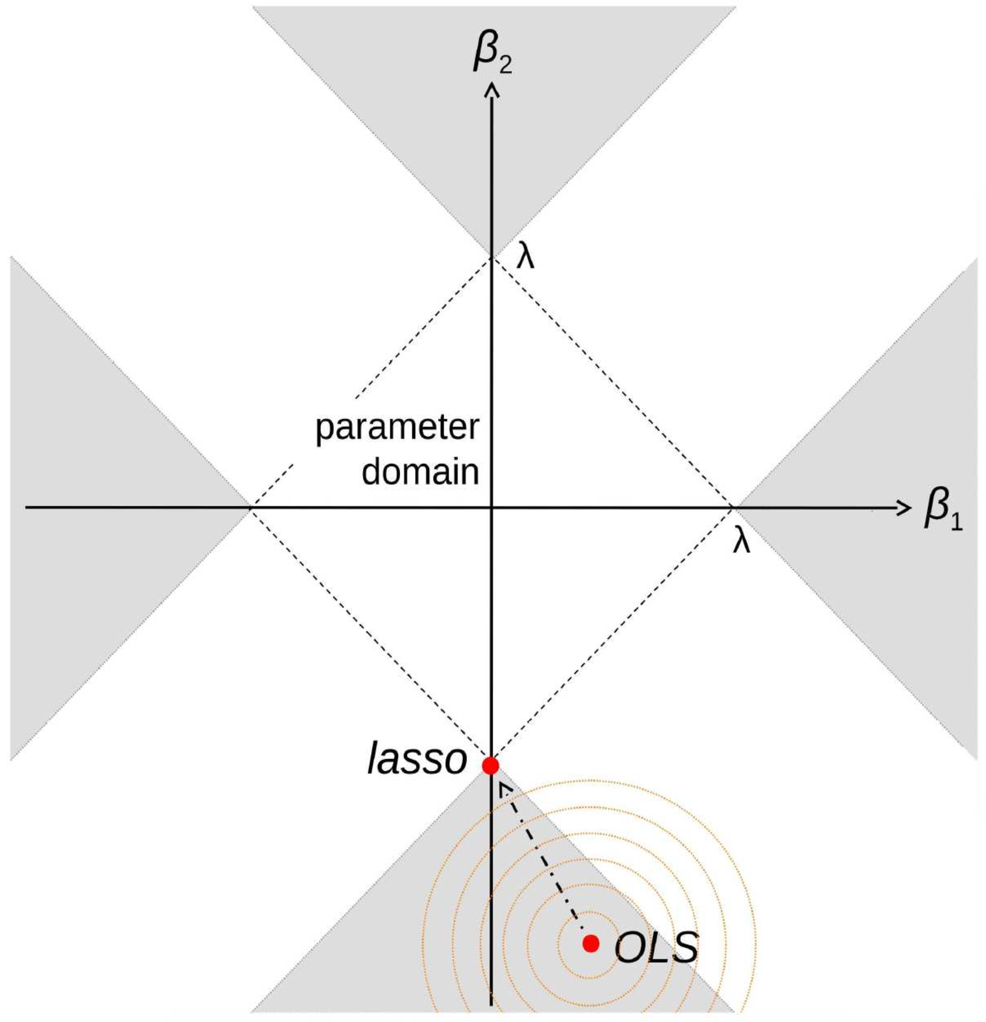
The selection property of the lasso is due to the fact that the diamond-shaped parameter constraint has its corners falling on the axes. For a point to lie on an axis, one coordinate needs to equal zero. The lasso regression estimator coincides with the point inside the diamond closest to the maximum likelihood estimator. This point may correspond to a corner of the diamond, in which case one of the coordinates (regression parameters) equals zero and, consequently, the lasso regression estimator does not select this element of [math]\bbeta[/math]. Figure illustrates the selection property for the case with [math]p=2[/math] and an orthonormal design matrix. An orthornormal design matrix yields level sets (orange dotted circles in Figure) of the sum-of-squares that are spherical and centered around the maximum likelihood estimate (red dot in Figure). For maximum likelihood estimates inside the grey areas the closest point in the diamond-shaped parameter domain will be on one of its corners. Hence, for these maximum likelihood estimates the corresponding lasso regression estimate will include on a single covariate in the model. The geometrical explanation of the selection property of the lasso regression estimator also applies to non-orthonormal design matrices and in dimensions larger than two. In particular, high-dimensionally, the sum-of-squares may be a degenerated ellipsoid, that can and will still hit a corner of the diamond-shaped parameter domain. Finally, note that a zero value of the lasso regression estimate does imply neither that the parameter is indeed zero nor that it will be statistically indistinguishable from zero.
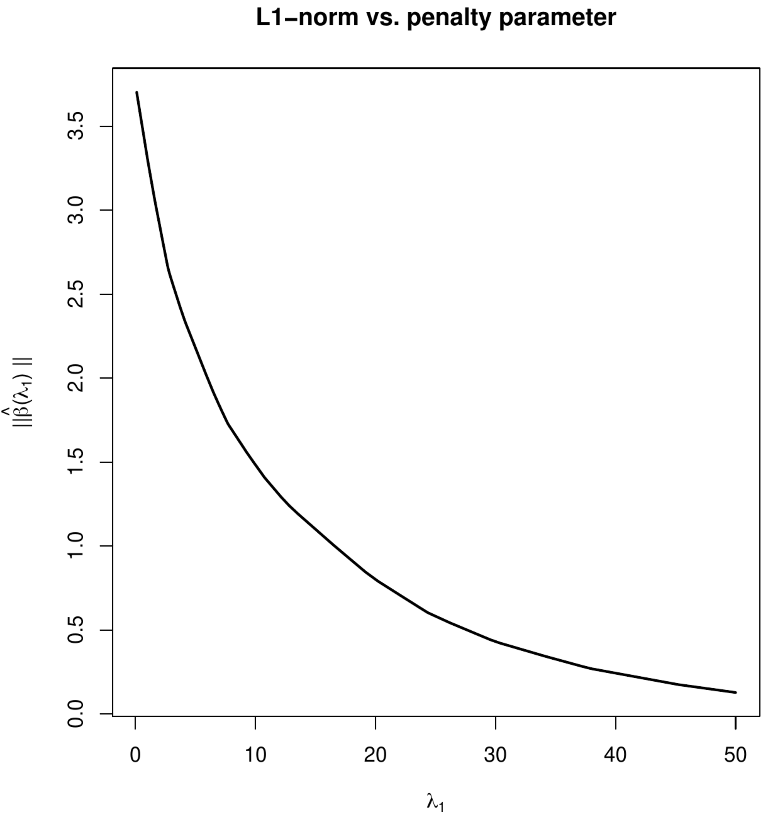
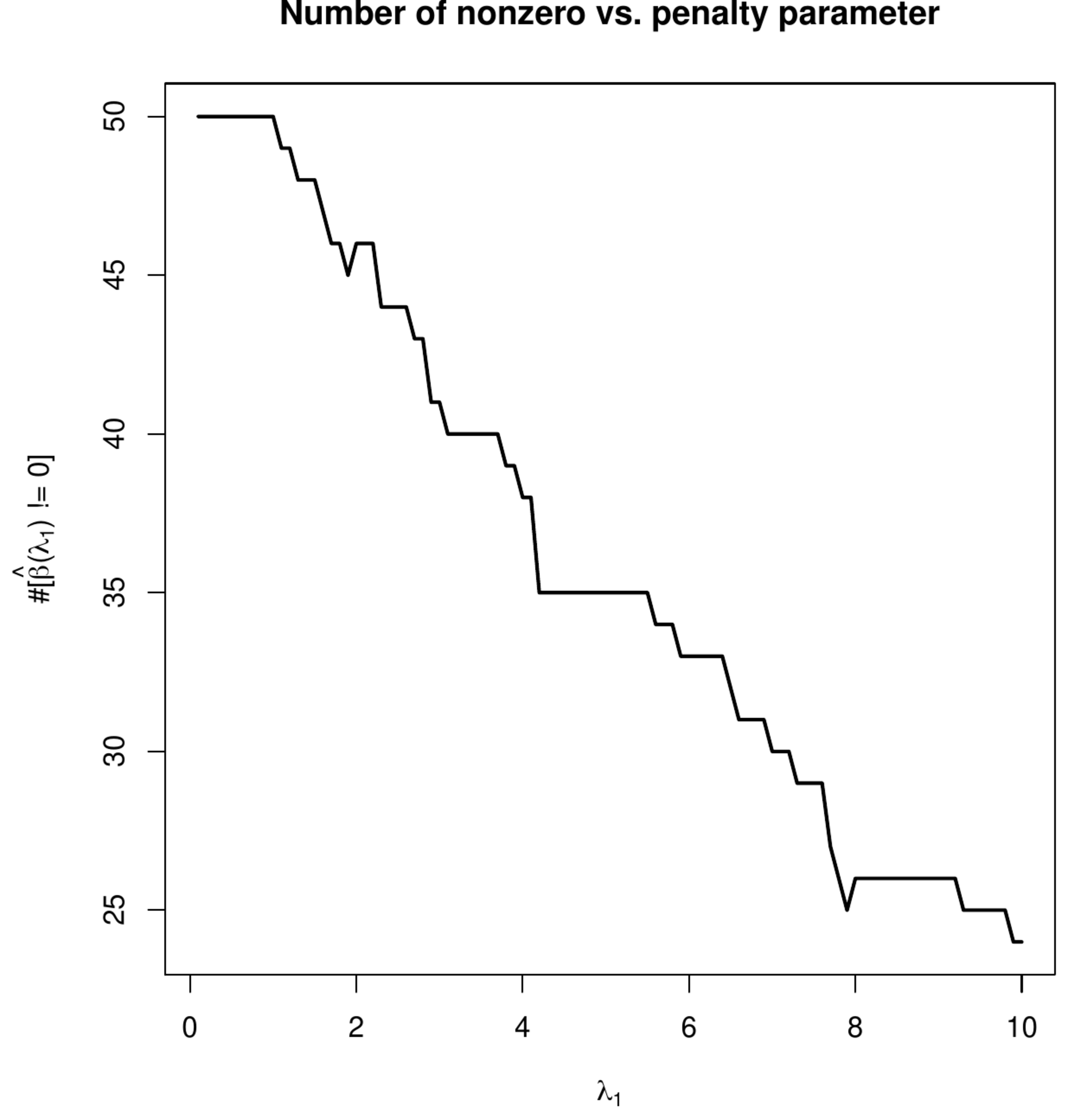
Larger values of the lasso penalty parameter [math]\lambda_1[/math] induce tighter parameter constraints. Consequently, the number of zero elements in the lasso regression estimator of [math]\bbeta[/math] increases as [math]\lambda_1[/math] increases. However, where [math]\| \hat{\bbeta}(\lambda_1) \|_1[/math] decreases monotonically as [math]\lambda_1[/math] increases (left panel of Figure for an example and Exercise Exercise), the number of non-zero coefficients does not. Locally, at some finite [math]\lambda_1[/math], the number of non-zero elements in [math]\hat{\bbeta}(\lambda_1)[/math] may temporarily increase with [math]\lambda_1[/math], to only go down again as [math]\lambda_1[/math] is sufficiently increased (as in the [math]\lambda_1 \rightarrow \infty[/math] limit the number of non-zero elements is zero, see the argumentation at the end of Section Analytic solutions ). The right panel of Figure illustrates this behavior for an arbitrary data set.
Contour plots of the sum-of-squares and the lasso regression loss (left and right panel, respectively). The dotted grey line represent level sets. The red line and dot represent the the location of minimum in both panels.
The attractiveness of the lasso regression estimator is in its simultaneous estimation and selection of parameters. For large enough values of the penalty parameter [math]\lambda_1[/math] the estimated regression model comprises only a subset of the supplied covariates. In high-dimensions (demanding a large penalty parameter) the number of selected parameters by the lasso regression estimator is usually small (relative to the total number of parameters), thus producing a so-called sparse model. Would one adhere to the parsimony principle, such a sparse and thus simpler model is preferable over a full model. Simpler may be better, but too simple is worse. The phenomenon or system that is to be described by the model need not be sparse. For instance, in molecular biology the regulatory network of the cell is no longer believed to be sparse [5]. Similarly, when analyzing brain image data, the connectivity of the brain is not believed to be sparse.
Maximum number of selected covariates
The number of parameter/covariates selected by the lasso regression estimator is bounded non-trivially. The cardinality (i.e. the number of included covariates) of every lasso estimated linear regression model is smaller than or equal to [math]\min\{n, p\}[/math] [6].
The nontrivial part of the inequality, that the number of selected variates [math]p[/math] does not exceed the sample size [math]n[/math], can be proven [7].
If [math]p \gt n[/math] and [math]\hat{\bbeta}(\lambda_1)[/math] is a minimizer of the lasso regresssion loss function (\ref{form.lassoLossFunction}), then [math]\hat{\bbeta}(\lambda_1)[/math] has at most [math]n[/math] non-zero entries.
Show Proof
In the high-dimensional setting, when [math]p[/math] is large compared to [math]n[/math] small, this implies a considerable dimension reduction. It is, however, somewhat unsatisfactory that it is the study design, i.e. the inclusion of the number of samples, that determines the upperbound of the model size.
General References
van Wieringen, Wessel N. (2021). "Lecture notes on ridge regression". arXiv:1509.09169 [stat.ME].
References
- Tibshirani, R. (1996).Regularized shrinkage and selection via the lasso.Journal of the Royal Statistical Society B, 58(1), 267--288
- Tibshirani, R. J. (2013).The lasso problem and uniqueness.Electronic Journal of Statistics, 7, 1456--1490
- 3.0 3.1 Rosset, S. and Zhu, J. (2007).Piecewise linear regularized solution paths.The Annals of Statistics, pages 1012--1030
- Leng, C., Lin, Y., and Wahba, G. (2006).A note on the lasso and related procedures in model selection.Statistica Sinica, pages 1273--1284
- Boyle, E. A., Li, Y. I., and Pritchard, J. K. (2017).An expanded view of complex traits: from polygenic to omnigenic.Cell, 169(7), 1177--1186
- Bühlmann, P.; Van De Geer, S. (2011). Statistics for High-Dimensional Data: Methods, Theory and Applications. Springer Science & Business Media.
- 7.0 7.1 7.2 Osborne, M. R., Presnell, B., and Turlach, B. A. (2000).On the lasso and its dual.Journal of Computational and Graphical Statistics, 9(2), 319--337
