Exercises

To view all exercises, please subscribe to guide

AAdmin

May 01'23

The loss due to a fire in a commercial building is modeled by a random variable [math]X[/math] with density function

[[math]] f(x) = \begin{cases} 0.005(20 − x), \, 0\lt x \lt 20 \\ 0, \, \textrm{otherwise.} \end{cases} [[/math]]

Given that a fire loss exceeds 8, calculate the probability that it exceeds 16.

1/25
1/9
1/8
1/3
3/7

AAdmin

May 01'23

A group insurance policy covers the medical claims of the employees of a small company. The value, [math]V[/math], of the claims made in one year is described by [math]V = 100,000Y[/math] where [math]Y[/math] is a random variable with density function

[[math]] f(y) = \begin{cases} k(1-y)^4, \, 0\lt y \lt 1 \\ 0, \, \textrm{otherwise} \end{cases} [[/math]]

where [math]k[/math] is a constant. Calculate the conditional probability that [math]V[/math] exceeds 40,000, given that [math]V[/math] exceeds 10,000.

0.08
0.13
0.17
0.20
0.51

AAdmin

May 01'23

An insurance policy pays for a random loss [math]X[/math] subject to a deductible of [math]C[/math], where [math]0 \lt C \lt 1[/math] . The loss amount is modeled as a continuous random variable with density function

[[math]] f(x) = \begin{cases} 2x, \, 0 \lt x \lt 1 \\ 0, \, \textrm{otherwise.} \end{cases} [[/math]]

Given a random loss [math]X[/math], the probability that the insurance payment is less than 0.5 is equal to 0.64. Calculate [math]C[/math].

0.1
0.3
0.4
0.6
0.8

AAdmin

May 01'23

An insurance policy pays 100 per day for up to three days of hospitalization and 50 per day for each day of hospitalization thereafter. The number of days of hospitalization, [math]X[/math], is a discrete random variable with probability function

[[math]] \operatorname{P}[X=k] = \begin{cases} \frac{6-k}{15}, \, k =1,2,3,4,5 \\ 0, \, \textrm{Otherwise.} \end{cases} [[/math]]

Determine the expected payment for hospitalization under this policy.

123
210
220
270
367

AAdmin

May 01'23

An auto insurance company insures an automobile worth 15,000 for one year under a policy with a 1,000 deductible. During the policy year there is a 0.04 chance of partial damage to the car and a 0.02 chance of a total loss of the car. If there is partial damage to the car, the amount [math]X[/math] of damage (in thousands) follows a distribution with density function

[[math]] f(x) = \begin{cases} 0.5003e^{− x /2}, \, 0 \lt x \lt 15 \\ 0, \, \textrm{Otherwise.} \end{cases} [[/math]]

Calculate the expected claim payment.

320
328
352
380
540

AAdmin

May 01'23

An insurer's annual weather-related loss, [math]X[/math], is a random variable with density function

[[math]] f(x) = \begin{cases} \frac{2.5(200)^{2.5}}{x^{3.5}}, \, x\gt200 \\ 0, \, \textrm{Otherwise.} \end{cases} [[/math]]

Calculate the difference between the 30^th and 70^th percentiles of [math]X[/math].

35
93
124
231
298

AAdmin

May 01'23

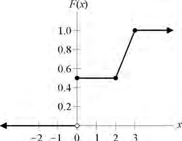
A man purchases a life insurance policy on his 40th birthday. The policy will pay 5000 if he dies before his 50th birthday and will pay 0 otherwise. The length of lifetime, in years from birth, of a male born the same year as the insured has the cumulative distribution function

[[math]] F(t) = \begin{cases} 1-\exp(\frac{1-1.1^t}{1000}), \, t \gt 0 \\ 0, \, \textrm{Otherwise.} \end{cases} [[/math]]

Calculate the expected payment under this policy.

333
348
421
549
574

AAdmin

May 01'23

The figure below shows the cumulative distribution function of a random variable, [math]X[/math].

Calculate [math]\operatorname{E}(X)[/math].

0.00
0.50
1.00
1.25
2.50

AAdmin

May 01'23

Damages to a car in a crash are modeled by a random variable with density function

[[math]] f(x) = \begin{cases} c(x^2 − 60x + 800), \, 0 \lt x \lt 20 \\ 0, \, \textrm{otherwise} \end{cases} [[/math]]

where [math]c[/math] is a constant. A particular car is insured with a deductible of 2. This car was involved in a crash with resulting damages in excess of the deductible.

Calculate the probability that the damages exceeded 10.

0.12
0.16
0.20
0.26
0.78

AAdmin

May 01'23

The distribution of the size of claims paid under an insurance policy has probability density function

[[math]] f(x) = \begin{cases} cx^a, \, 0 \lt x \lt 5 \\ 0, \, \textrm{otherwise} \end{cases} [[/math]]

Where [math]a \gt 0[/math] and [math]c \gt 0 [/math]. For a randomly selected claim, the probability that the size of the claim is less than 3.75 is 0.4871.

Calculate the probability that the size of a randomly selected claim is greater than 4.

0.404
0.428
0.500
0.572
0.596